The Long-Term Control Plan-EZ (LTCP-EZ) Template: A Planning Tool for CSO Control in Small Communities

United States

Environmental Protection

Agency

Office of Water (4203)

Washington, DC 20460

www.epa.gov/npdes/cso

EPA-833-R-07-005

May 2007

The Long-Term Control Plan-

EZ (LTCP-EZ) Template:

A Planning Tool for CSO Control

in Small Communities

The LTCP-EZ Template: A Planning Tool for CSO Control in Small Communities

Table of Contents

BACKGROUND...................................................................................................................................................................... 1

INSTRUCTIONS: FORM LTCP-EZ ........................................................................................................................................ 5

General Information ................................................................................................................................................................ 6

Nine Minimum Controls (Schedule 1—NMC) ......................................................................................................................... 6

Sensitive Areas ....................................................................................................................................................................... 6

Water Quality Considerations ................................................................................................................................................. 7

System Characterization (Schedule 2—MAP) ........................................................................................................................ 8

Public Participation (Schedule 3—PUBLIC PARTICIPATION)............................................................................................. 10

CSO Volume (Schedule 4—CSO VOLUME)........................................................................................................................ 11

Evaluation of CSO Controls (Schedule 5—CSO CONTROL) .............................................................................................. 11

Affordability (Schedule 6—CSO AFFORDABILITY) ............................................................................................................. 11

Recommended CSO Control Plan ........................................................................................................................................ 12

INSTRUCTIONS: SCHEDULE 4 – CSO VOLUME.............................................................................................................. 14

Sub-Sewershed Area ............................................................................................................................................................ 16

Runoff.................................................................................................................................................................................... 16

Dry Weather Flow Within the CSS........................................................................................................................................ 17

Peak Wet Weather Flow ....................................................................................................................................................... 17

Overflow ................................................................................................................................................................................ 17

Diversion ............................................................................................................................................................................... 17

Conveyance .......................................................................................................................................................................... 18

Treatment.............................................................................................................................................................................. 19

CSO Volume ......................................................................................................................................................................... 20

INSTRUCTIONS: SCHEDULE 5 – CSO CONTROL .......................................................................................................... .21

Conveyance and Treatment at the WWTP ........................................................................................................................... 23

Inflow Reduction – Residential.............................................................................................................................................. 23

Sewer Separation.................................................................................................................................................................. 24

Off-Line Storage.................................................................................................................................................................... 24

Summary of Controls and Costs ........................................................................................................................................... 24

INSTRUCTIONS: SCHEDULE 6 – CSO AFFORDABILITY ................................................................................................ 26

Phase I Residential Indicator ................................................................................................................................................ 27

Current Costs ........................................................................................................................................................................ 27

Projected Costs (Current Dollars) ......................................................................................................................................... 27

Cost Per Household .............................................................................................................................................................. 28

Median Household Income (MHI) ......................................................................................................................................... 28

Residential Indicator.............................................................................................................................................................. 29

Phase II Permittee Financial Capability Indicators................................................................................................................ 29

Debt Indicators ...................................................................................................................................................................... 30

Overall Net Debt.................................................................................................................................................................... 30

Socioeconomic Indicators ..................................................................................................................................................... 31

Unemployment Rate ............................................................................................................................................................. 31

Median Household Income ................................................................................................................................................... 32

Financial Management Indicators ......................................................................................................................................... 32

Property Tax and Collection Rate ......................................................................................................................................... 33

Matrix Score: Analyzing Permittee Financial Capability Indicators....................................................................................... 33

GLOSSARY ..........................................................................................................................................................................35

REFERENCES......................................................................................................................................................................39

APPENDIX A—ONE-HOUR THREE-MONTH RAINFALL INTENSITIES FOR SCHEDULE 4 – CSO VOLUME

APPENDIX B—HYDRAULIC CALCULATIONS WITHIN LTCP-EZ SCHEDULES 4 AND 5

APPENDIX C—COST ESTIMATES FOR SCHEDULE 5 – CSO CONTROL

The LTCP-EZ Template: A Planning Tool for CSO Control in Small Communities

LIST OF ACRONYMS

AF – Annualization Factor

BOD – Bioche

mical Oxygen Demand

CPH – Costs per Household

CPI – Consumer Price Index

CSO – Combined Sewer Overflow

CSS – Combined Sewer System

DO – Dissolved Oxygen

DMR – Discharge Monitoring Report

DWF – Dry Weather Flow

EPA – Environmental Protection Agency

FWS – Fish and Wildlife Service

I/I – Inflow/Infiltration

IR – Interest Rate

LTCP – Long-term Control Plan

MG – Million Gallons

MGD – Million Gallons per Day

MHI – Median Household Income

NOAA – National Oceanic and Atmospheric Administration

NMC – Nine Minimum Controls

NMFS – National Marine Fisheries Service

NPDES – National Pollutant Discharge Elimination System

POTW – Publicly Owned Treatment Works

TMDL – Total Maximum Daily Load

TSS – Total Suspended Solids

WQS – Water Quality Standards

WWT – Wastewater Treatment

WWTP – Wastewater Treatment Plant

The LTCP-EZ Template: A Planning Tool for CSO Control in Small Communities

BACKGROUND

What is the LTCP-EZ Template and what is its Purpose?

The combined sewer overflow (CSO) Long-Term Control Plan (LTCP) Template for Small Communities (termed the

“LTCP-EZ Template”) is a planning tool for small communities that have requirements to develop a LTCP to address

CSOs. The LTCP-EZ Template provides a framework for organization and completion of a LTCP that builds upon existing

controls and leads to the elimination or control of CSOs in accordance with the federal Clean Water Act. Use of the LTCP-

EZ Template and completion of the forms and schedules associated with the LTCP-EZ Template can produce a Draft

LTCP.

The LTCP-EZ Template consists of FORM LTCP-EZ and related schedules and instructions. It provides a starting place

and a framework for small communities for organization and analysis of basic information that is central to effective CSO

control planning. Specifically, FORM LTCP-EZ and Schedules 1 – NINE MINIMUM CONTROLS, 2 – MAP, and 3 –

PUBLIC PARTICIPATION allow organization of some of the basic information required to comply with the CSO policy.

Schedule 4 – CSO VOLUME provides a process for assessing CSO control needs under the “presumption approach.” It

allows the permittee or other user (the term permittee will be used throughout this document, but the term should be

interpreted to include any users of the LTCP-EZ Template) to estimate a target volume of combined sewage that needs to

be stored, treated, or eliminated. Schedule 5 – CSO CONTROL enables the permittee to evaluate the ability of a small but

widely used set of CSO controls to meet the reduction target. Finally, Schedule 6 – CSO AFFORDABILITY provides an

EPA affordability analysis to determine the community’s financial capabilities. Permittees are free to use FORM LTCP-EZ

and as many schedules as needed to meet their local needs and requirements. FORM LTCP-EZ and its schedules are

available in hard copy format or as computer-based spreadsheets.

This publication provides background information on the CSO Control Policy and explains the data and information

requirements, technical assessments, and calculations that are addressed in the LTCP-EZ Template and are necessary

for its application.

What is the Relationship Between LTCP-EZ and the CSO Control Policy?

The Clean Water Act Section 402(q) and the CSO Control Policy (EPA 830-B-94-001) (http://www.epa.gov/npdes/

pubs/owm0111.pdf) require permittees with combined sewer systems (CSSs) that have CSOs to undertake a process to

accurately characterize their sewer systems, demonstrate implementation of the nine minimum controls (NMC), and

develop a LTCP. The U.S. Environmental Protection Agency (EPA) recognizes that resource constraints make it difficult

for small communities to prepare a detailed LTCP. Section I.D of the CSO Control Policy states that:

The scope of the LTCP, including the characterization, monitoring and modeling, and evaluation of alternatives

portions of the Policy may be difficult for some small CSSs. At the discretion of the NPDES Authority, jurisdictions with

populations under 75,000 may not need to complete all of the formal steps outlined in Section II.C. of this Policy, but

should be required through their permits or other enforceable mechanisms to comply with the nine minimum control

(II.B), public participation (II.C.2), and sensitive areas (II.C.3) portions of this Policy. In addition, the permittee may

propose to implement any of the criteria contained in this Policy for evaluation of alternatives described in II.C.4.

Following approval of the proposed plan, such jurisdictions should construct the control projects and propose a

monitoring program sufficient to determine whether water quality standards are obtained and designated use are

protected.

EPA developed the LTCP-EZ Template, in part, because it recognizes that expectations for the scope of the LTCP for

small communities may be different than for larger communities. However, the LTCP-EZ Template does not replace the

statutory and regulatory requirements applicable to CSOs; those requirements continue to apply to the communities using

this template. Nor does its use ensure that a community using the LTCP-EZ Template will necessarily be deemed to be in

compliance with those requirements. It is hoped, however, that use of the LTCP-EZ Template will facilitate compliance by

small communities with those legal requirements and simplify the process of developing a LTCP.

IMPORTANT NOTE: Each permittee should discuss use of the LTCP-EZ Template and coordinate with the

appropriate regulatory authority or with their permit writer and come to an agreement with the permitting authority

on whether use of the LTCP-EZ Template or components thereof is acceptable for the community.

BACKGROUND

Who Should Use the LTCP-EZ Template?

The LTCP-EZ Template is designed as a planning tool for use by small communities that have not developed LTCPs and

have limited resources to invest in CSO planning. It is intended to assist small communities in developing an LTCP that

will build on NMC implementation and lead to additional elimination and reduction of CSOs where needed. CSO

communities using the LTCP-EZ Template should recognize that this planning tool

is for use in facility-level planning. Use

of the LTCP-Template should be based upon a solid understanding of local conditions that cause CSOs. CSO

communities should familiarize themselves with all of the technical analyses required by the LTCP-EZ planning process.

CSO communities should obtain the assistance of qualified technical professionals (e.g., qualified engineer, hydraulic

expert, etc.) to assist with completion of analyses if they are unable to complete the LTCP-EZ Template on their own.

More detailed design studies will be required for construction of new facilities.

The LTCP-EZ Template is particularly well suited for small CSO communities that have relatively uncomplicated CSSs.

The use of the LTCP-EZ Template may or may not be suitable for large CSO communities with populations of greater

than 75,000 or even for the largest of the small CSO communities. Large CSO communities and small CSO communities

that have many CSO outfalls and complex systems may need to take a more sophisticated approach to LTCP

development, and this should be evaluated by consultation with regulators as discussed above.

Because the LTCP-EZ uses a specific approach to analyzing the CSS and controlling CSOs, these instructions

emphasize the need for dialogue between small CSO communities and their appropriate regulatory authority on use of the

LTCP-EZ Template. Both the permittee and the permitting agency should evaluate the applicability of the LTCP-EZ.

The LTCP-EZ Template is intended to provide a very simple assessment of CSO control needs. As such, it may reduce

effort and costs associated with CSO control development. However, permittees should bear in mind that due to its

simple nature, the LTCP-EZ Template may not evaluate a full range of potential CSO control approaches.

What Approach is used in the LTCP-EZ Template?

Schedules 4 - CSO VOLUME and Schedule 5 – CSO CONTROL use the “presumption approach” described in the CSO

Control Policy to quantify the volume of combined sewage that needs to be stored, treated, or eliminated. The CSO

Control Policy describes two alternative approaches available to communities to establish that their LTCPs are adequate

to meet the water quality-based requirements of the Clean Water Act: the “presumption approach” and the

“demonstration approach” (Policy Section II.C.4.a.) The “presumption approach” sets forth criteria that, when met, are

presumed to provide an adequate level of control to meet the water quality-based requirements:

… would be presumed to provide an adequate level of control to meet water quality-based requirements of the Clean

Water Act, provided the permitting authority determines that such presumption is reasonable in light of data and

analysis conducted in the characterization, monitoring, and modeling of the system and the consideration of sensitive

areas described above (in Section II.C.4.a). These criteria are provided because data and modeling of wet weather

events often do not give a clear picture of the level of CSO controls necessary to protect WQS (water quality

standards).

The estimation of a target volume of combined sewage that needs to be stored, treated, or eliminated in Schedule 4 –

CSO VOLUME in the LTCP-EZ Template uses the “presumption approach” described in the CSO Control Policy.

The permittee is advised to consider a limited rainfall and flow monitoring program. Performance of simple regression

analyses (e.g., rainfall vs. flow response) can be used to refine the LTCP-EZ Template output and increase confidence in

the sizing of controls generated using the LTCP-EZ Template. The permittee can refer to EPA’s Combined Sewer

Overflows Guidance for Monitoring and Modeling (EPA 832-B-99-002, January 1999)

(http://www.epa.gov/npdes/pubs/sewer.pdf

) for examples of this approach to rainfall response characterization.

Selected criterion under the “presumption approach” used in the LTCP-EZ Template

The CSO Control Policy allows a community’s LTCP to meet any one of three criteria to be “presumed to provide an

adequate level of control . . . .” The LTCP-EZ Template uses one of those criteria only, set forth in section II.C.4.a.i. as

follows:

The LTCP-EZ Template: A Planning Tool for CSO Control in Small Communities

No more than an average of four overflow events per year, provided that the permitting authority may allow up to two

additional overflow events per year. For the purpose of this criterion, an overflow event is one or more overflows from

a CSS as the result of a precipitation event that does not receive the minimum treatment specified below.

The “minimum treatment specified” with respect to the criteria in Section II.C.4.a.i. of the CSO Control Policy is defined as:

• Primary clarification; removal of floatable and settleable solids may be achieved by any combination of treatment

technologies or methods that are shown to be equivalent to primary clarification;

• Solids and floatable disposal; and

• Disinfection of effluent, if necessary, to meet water quality standards, protect designated uses, and protect human

health, including removal of harmful disinfection chemical residuals, where necessary.

This approach is used because the criteria set forth under the “presumption approach” lend themselves to quantification

with simple procedures and a standardized format.

Calculations within Schedule 4 - CSO VOLUME and Schedule 5 – CSO CONTROL

Schedules 4 and 5 use design storm conditions to assess the degree of CSO control required to meet the average of four

overflow events per year criteria. Design storms are critical rainfall conditions that occur with a predictable frequency.

They are used with simple calculations to quantify the volume of combined sewage to be stored, treated, or eliminated to

meet the criterion of no more than four overflows per year, on average. The “design storm” is explained in further detail in

the instructions for Schedule 4 – CSO VOLUME.

The LTCP-EZ Template also provides permittees with simple methods to assess the costs and effectiveness of a variety

of CSO control alternatives in Schedule 5 – CSO CONTROL.

Use of the “presumption approach” and the use of Schedules 4 and 5 may not be appropriate for every community. Some

states have specific requirements that are inconsistent with Schedules 4 and 5. Also use of the LTCP-EZ Template does

not preclude permitting authorities from requesting clarification or requiring additional information. Permittees should

consult with the appropriate regulatory authority to determine whether or not the “presumption approach” and its

interpretation under Schedules 4 and 5 are appropriate for their local circumstances.

How is Affordability Assessed?

The CSO Financial Capability Assessment Approach outlined in EPA’s Combined Sewer Overflows–Guidance for

Financial Capability Assessment and Schedule Development (EPA 832-B-97-004) is contained in Schedule 6 – CSO

AFFORDABILITY. (http://www.epa.gov/npdes/pubs/csofc.pdf

)

SUMMARY

The LTCP-EZ Template is an optional CSO control planning tool for small communities. It provides one approach for

assembling and organizing the information required in an LTCP. FORM LTCP-EZ and Schedules 1 (Nine Minimum

Controls), 2 (Map) and 3 (Public Participation) allow organization of some of the basic elements to comply with the CSO

policy. Schedule 4 – CSO VOLUME allows the permittee to estimate a target volume of combined sewage that needs to

be stored, treated, or eliminated. Schedule 5 – CSO CONTROL enables the permittee to evaluate the ability of a small but

widely used set of CSO controls to meet the reduction target. FORM LTCP-EZ and its schedules are available in hard

copy format or as computer-based spreadsheets. Schedule 6 – CSO AFFORDABILITY provides an EPA affordability

analysis to assess the community’s financial capabilities.

The CSO Control Policy and all of EPA’s CSO guidance documents can be found at the following link:

http://cfpub.epa.gov/npdes/home.cfm?program_id=5

This page is intentionally blank.

The LTCP-EZ Template: A Planning Tool for CSO Control in Small Communities

GENERAL INSTRUCTIONS: LTCP-EZ TEMPLATE

FORM LTCP-EZ encompasses all of the information that most small CSO communities need to develop a draft LTCP.

This includes characterization of the CSS, documentation of NMC implementation, documentation of public participation,

identification and prioritization of sensitive areas where present, and evaluation of CSO control alternatives and

affordability.

The LTCP-EZ Template includes a form (Form LTCP-EZ) and schedules for

organizing the following information:

Using the Electronic Forms for the

LTCP-EZ Template

The electronic version of the LTCP-EZ

Template forms have cells that link data in

one worksheet to other worksheets, and

therefore it is important that you work on

the worksheets in order and fill in all of the

pertinent information. If you are filling in the

LTCP-EZ Template forms by hand, you will

have to copy the information from one form

into the other.

• General information about the CSS, the wastewater treatment plant

(WWTP) and the community served

• NMC implementation activities (Schedule 1 – NMC)

• Sensitive Area considerations

• Water quality considerations

• System characterization, including a map of the CSS (Schedule 2 –

MAP)

• Public participation activities (Schedule 3 – PUBLIC

PARTICIPATION)

• CSO volume that needs to be controlled (Schedule 4 – CSO

VOLUME)

• Evaluation of CSO controls (Schedule 5 – CSO CONTROL)

• Affordability analysis (Schedule 6 – CSO AFFORDABILITY)

• Recommended CSO Control Plan, including financing plan and implementation schedule.

Permittees intending to use the LTCP-EZ Template should assemble the following information:

• The NPDES permit.

• General information about the CSS and the WWTP including sub-

sewershed delineations for individual CSO outfalls and the

capacities of hydraulic control structures, interceptors, and

wastewater treatment processes.

• Relevant engineering studies and facility plans for the sewer system

and WWTP if available.

• Maps for sewer system.

• General demographic information for the community.

• General financial information for the community.

• A summary of historical actions and current programs that represent

implementation of the NMCs. The NMC are controls that can reduce

CSOs and their effects on receiving waters, do not require significant

engineering studies or major construction, and can be implemented in a relatively short period (e.g., less than

approximately two years).

Guidance from EPA

EPA has developed the Combined Sewer

Overflows Guidance For Long-Term

Control Plan (EPA 832-B-95-002)

(http://www.epa.gov/npdes/pubs/owm0272.pdf

)

document to assist municipalities with

developing a long-term control plan that

includes technology-based and water

quality-based control measures that are

technically feasible, affordable, and

consistent with the CSO Control Policy.

• Information on water quality conditions in local waterbodies that receive CSO discharges.

Once complete, the LTCP-EZ Template (FORM LTCP-EZ with accompanying schedules) can serve as a draft LTCP for a

small community. All of the schedules provided in the LTCP-EZ Template may not be appropriate for every permittee. It

may not be necessary to use all of the schedules provided in this template in order to complete a draft LTCP. In addition,

permittees can attach the relevant documentation to FORM LTCP-EZ in a format other than the schedules provided in the

LTCP-EZ Template.

INSTRUCTIONS: FORM LTCP-EZ

INSTRUCTIONS: FORM

LTCP-EZ

General Information

Line 1 – Community Information.

Enter the community name,

National Pollutant Discharge

Elimination System (NPDES) permit

number, owner/operator, facility

name, mailing address, telephone

number, fax number, and email

address, as well as the date.

Line 2 – System Type. Identify the

type of system that this LTCP is

being developed for:

• NPDES permit for a CSS with a

WWTP or

• NPDES permit for a CSS

without a WWTP

Line 3a – CSS. Enter the total area

served by the CSS in acres.

Line 3b – Enter the number of

permitted CSO outfalls.

Line 4 – WWTP. Enter the following

information for WWTP capacity in

million gallons per day (MGD).

• Line 4a – Primary treatment

capacity in MGD.

• Line 4b – Secondary treatment

capacity in MGD.

• Line 4c – Average dry weather

flow in MGD. Dry weather flow

(DWF) is the base sanitary flow

delivered to a CSS in periods

without rainfall or snowmelt. It

represents the sum of flows

from homes, industry,

commercial activities, and

infiltration. Dry weather flow is

usually measured at the WWTP

and recorded on a Discharge

Monitoring Report (DMR).

For the purposes of the

calculation in the LTCP-EZ

Template, base

sanitary flow is

assumed to be constant. There

is no need to adjust entries for

diurnal or seasonal variation.

Nine Minimum Controls

The CSO Control Policy (Section

II.B.) sets out nine minimum

controls, which are technology-

based controls that communities are

expected to use to address CSO

problems, without undertaking

extensive engineering studies or

significant construction costs,

before long-term measures are

taken. Permittees with CSSs

experiencing CSOs should have

implemented the NMC with

appropriate documentation by

January 1, 1997.The NMC are:

• NMC 1. Proper operations and

regular maintenance programs

for the CSS and CSO outfalls.

• NMC 2. Maximum use of the

CSS for storage.

• NMC 3. Review and

modification of pretreatment

requirements to ensure CSO

impacts are minimized.

• NMC 4. Maximizing flow to the

publicly-owned treatment works

(POTW) for treatment.

• NMC 5. Prohibition of CSOs

during dry weather.

• NMC 6. Control of solid and

floatable materials in CSOs.

• NMC 7. Pollution prevention

• NMC 8. Public notification to

ensure that the public receives

adequate notification of CSO

occurrences and CSO impacts.

• NMC 9. Monitoring to effectively

characterize CSO impacts and

the efficacy of CSO controls.

Line 5 – NMC. Permittees can

attach previously submitted

documentatio

n on NMC

implementation, or they can use

Schedule 1 – NMC to document

NMC activities. Please check the

appropriate box on Line 5 to

indicate how documentation of NMC

implementation is provided.

If Schedule 1 – NMC is used,

please do

cument the activities

taken to implement the NMC.

Documentation should include

information that demonstrates:

• The alternatives considered

for each minimum control

• The actions selected and

the reasons for their

selection

• The selected actions

already implemented

• A schedule showing

additional steps to be taken

• The effectiveness of the

minimum controls in

reducing/eliminating water

quality impacts (in reducing

the volume, frequency, and

impact of CSOs).

Leave the description blank if no

activities have been undertaken for

a particular NMC. See EPA’s

Combined Sewer Overflows

Guidance for Nine Minimum

Controls (EPA 832-B-95-003) for

examples of NMC activities and for

further guidance on NMC

documentation

(http://www.epa.gov/npdes/pubs/

owm0030.pdf).

Sensitive Areas

Permittees are expected to give the

highest priority to controlling CSOs

to sensitive areas. (CSO Control

Policy Section II.C.3.) Permittees

should identify all sensitive

waterbodies and the CSO outfalls

that discharge to them. The

identification of sensitive areas can

direct the selection of CSO control

alternatives. In accordance with the

CSO Control Policy, the LTCP

should give the highest priority to

the prohibition of new or

significantly increased overflow

(whether treated or untreated) to

designated sensitive areas.

Sensitive areas, as identified in the

CSO Control Policy, include:

The LTCP-EZ Template: A Planning Tool for CSO Control in Small Communities

• Outstanding National

Resource Waters. These are

waters that have been

designated by some (but not all)

states: “[w]here high quality

waters constitute an

outstanding National resource,

such as waters of National

Parks, State parks and wildlife

refuges, and waters of

exceptional recreational or

ecological significance, that

water quality shall be

maintained and protected” (40

CFR 122.12(a)(3)). Tier III

Waters and Class A Waters are

sometimes used to designate

Outstanding National Resource

Waters. State water quality

standards authorities are the

best source of information on

the presence of identified

Outstanding National Resource

Waters.

• National Marine Sanctuaries.

The National Oceanic and

mospheric Administration

(NOAA) is the trustee for the

nation's system of marine

protected areas, to conserve,

protect, and enhance their

biodiversity, ecological integrity

and cultural legacy. Information

on the location of National

Marine Sanctuaries can be

found at:

http://sanctuaries.noaa.gov/

• Waters with Threatened or

Endangered Species and

their Habitat. Information on

threatened and endangered

species can be identified by

contacting the Fish and Wildlife

Service (FWS), NOAA

Fisheries, or State or Tribal

Heritage Center or by checking

resources such as the FWS

website at http://www.fws.gov/

endangered/wildlife.html. If

there are listed species in the

area, contact the appropriate

local agency to determine if the

listed species could be affected

or if any critical habitat areas

have been designated in

waterbodies that receive CSO

discharges.

• Waters with Primary Contact

Recreation: State water quality

standards authorities are the

best source of information on

the location of waters

designated for primary contact

recreation.

• Public Drinking Water Intakes

or their Designated

Protection Areas. State water

quality standards and water

supply authorities are the best

source of information on the

location of public drinking water

intakes or their designated

protection areas. EPA’s Report

to Congress – Impacts and

Control of CSOs and SSOs

identified 59 CSO outfalls in

seven states located within one

mile upstream of a drinking

water intake (EPA 2004).

• Shellfish Beds. Shellfish

harvesting can be a designated

use of a waterbody. State water

quality standards authorities are

a good source of information on

the location of waterbodies that

are protected for shellfish

harvesting. In addition, the

National Shellfish Register of

Classified Estuarine Waters

provides a detailed analysis of

the shellfish growing areas in

coastal waters of the United

States. Information on the

location of shellfish beds can be

found at http://gcmd.nasa.gov/

records/GCMD_NOS00039.

html

Contact the appropriate state and

federal agencies to determine if

sensitive areas are present in the

area of the CSO. EPA recommends

that the permittee attach all

documentation of research

regarding sensitive areas and/or

contacts with agencies providing

that information (including research

on agency websites) to the LTCP-

EZ Template forms. In addition, the

permittee is encouraged to attach

maps or other materials that provide

back-up information regarding the

evaluation of sensitive areas.

Line 6a – Indicate if sensitive areas

are present. Answer Yes or No. If

sensitive areas are present,

proceed to Line 6b and answer

questions 6b, 6c, and 6d. Also

provide an explanation of how the

determination was made that

sensitive areas are present. If

sensitive areas are not present,

proceed to Line 7.

Line 6b – Enter the type(s) of

sensitive areas present (e.g., public

beach, drinking water intake) for

each CSO receiving water.

Line 6c – List the permitted CSO

outfall(s) that may be impacting the

sensitive areas. Add detail on

impacts where available (e.g., CSO

outfall is located within a sensitive

area, beach closures have occurred

due to overflows, etc.).

Line 6d – Are sensitive areas

impacted by CSO discharges?

Answer Yes or No. If sensitive

areas are present but not impacted

by CSO discharges, then provide

documentation on how the

determination was made and

proceed to Line 7.

More detailed study may be

necessary if sensitive

areas are present and

are

impacted by CSO discharges.

Under these circumstances, use of

the “presumption approach” in the

LTCP-EZ Template may not be

appropriate. The permittee should

contact the permitting authority for

further instructions on use of the

LTCP-EZ Template and/or the

“presumption approach”.

Water Quality

Considerations

The main impetus for

implementation of CSO controls is

attainment of water quality

standards, including designated

uses. Permittees are expected to be

knowledgeable about water quality

conditions in local waterbodies that

receive CSO discharges. At a

INSTRUCTIONS: FORM LTCP-EZ

minimum, permittees should check

to see if the local waterbodies have

been assessed under the 305(b)

program by the state water quality

standards agency as being “good”,

“threatened” or “impaired”.

Waters designated as impaired are

included on a state’s 303(d) list. A

total maximum daily load (TMDL) is

required for each pollutant causing

impairment. EPA’s recent Report to

Congress – Impacts and Control of

CSOs and SSOs (EPA 833-R-04-

001) identified the three causes of

reported 303(d) impairment most

likely to be associated with CSOs:

• Pathogens

• Organic enrichment leading to

low dissolved oxygen (DO)

• Sediment and siltation

Some states identify sources of

impairment, and the activities or

conditions that generate the

pollutants causin

g impairment (e.g.,

WWTPs or agricultural runoff).

CSOs are tracked as a source of

impairment in some but not all CSO

states.

If local waterbodies receiving CSO

discharges ar

e impaired, permittees

should check with the permitting

authority to determine whether or

not the pollutants associated with

CSOs are cited as a cause of

impairment, or if CSOs are listed as

a source of impairment. In addition,

permittees should check with the

permitting authority to see if a

TMDL study is scheduled for local

waterbodies to determine the

allocation of pollutant loads,

including pollutant loads in CSO

discharges.

The 305(b) water quality

assessment information can be

found at http://www.epa.gov/

waters/305b/index.html

. Note that

not all waters are assessed under

state programs.

A national summary on the status

of the TMDL program in each state

can be found at

http://www.epa.gov/owow/tmdl/

Note that not all waters are listed.

Line 7a – Indicate if local

waterbodi

es are listed by the

permitting authority as impaired.

Answer Yes or No. If No, then the

permittee may continue to Line 8.

Line 7b – Indicate the causes or

sources of impairment for each

impaired waterbody.

Line 7c – Indicate if a TMDL has

been scheduled to determine the

allocation of pollutant loads. Answer

Yes or No. If yes, provide the date.

If the identified waterbodies

have been assessed as

threatened or impaired

under the 305(b) program, and if

CSOs are cited as a source of

impairment or if the pollutants found

in CSOs are listed as a cause of

impairment, then CSOs likely cause

or contribute to a recognized water

quality problem. Under these

circumstances, permittees should

check with the permitting authority

to confirm that use of the LTCP-EZ

Template and/or the “presumption

approach” is appropriate.

If the waterbodies are not

designated by the permitting

authority as impaired or if the water

body is impaired but the CSO

discharges are not viewed as a

cause of the impairment, then the

permittee may continue with the

LTCP-EZ Template.

System Characterization

CSO control planning involves

consideration of the site-specific

nature of CSOs. The amount of

combined sewage flow that can be

conveyed to the WWTP in a CSS

depends on a combination of

regulator capacity, interceptor

capacity, pump station capacity,

and WWTP capacity. The LTCP-EZ

Template uses the term “CSO

hydraulic control capacity” as a

generic reference to these types of

flow controls. In any particular

system, one or more of these CSO

hydraulic control capacities may be

the limiting factor. If the community

has not previously carried out an

analysis of the peak capacity of

each portion of its CSS, it is strongly

suggested that the determination of

each CSO hydraulic control

capacity be carried out by

individual(s) experienced in such

hydraulic analyses. Communities

are particularly cautioned against

evaluating CSO regulator capacity

without considering interceptor

capacity as well, as the nominal

capacity of a given CSO regulator

may exceed that of its receiving

interceptor under the same peak

wet weather conditions.

To develop an adequate control

plan, the permittee needs to have a

thorough understanding of the

following:

• The extent of the CSS and

the number of CSO outfalls

• The interconnectivity of the

system

• The response of the CSS to

rainfall

• The water quality

characteristics of the CSOs

• The water quality impacts

that result from CSOs.

Of these, the first three

considerations are the most

important for small communities.

Communities using the LTCP-EZ

Template are encouraged to obtain

at least limited rainfall and system

flow data to allow the runoff

response calculated by the LTCP-

EZ approach to be checked against

actual system flow data.

Line 8 is used to indicate that a map

has been attached to the LTCP-EZ

Template. Lines 9-11 provide more

specific information about the CSS.

Information on Lines 9 through 11 is

organized by CSO outfall and sub-

sewershed.

Line 8 – General Location. Please

check the box on Line 8 to indicate

Schedule 2 – MAP is attached to

FORM LTCP-EZ. Schedule 2 –

The LTCP-EZ Template: A Planning Tool for CSO Control in Small Communities

MAP should include a map or

sketch of the CSS that shows the

following:

• Boundaries of the CSS service

area and, if different, total area

served by the sewer system

• CSO outfall locations

• Boundaries of individual sub-

sewersheds within the CSS

that drain to a CSO outfall

• Location of major hydraulic

control points such as CSO

regulators (weirs, diversion

structures, etc.) and pump

stations

• Location of major sewer

interceptors (show as pathways

to the WWTP)

• WWTP, if present

• Waterbodies

Delineation of the boundaries of the

CSS and individual sub-sewersheds

is very import

ant. Delineation is

most often done by hand with sewer

maps, street maps, contours, and

the location of key hydraulic control

points such as regulators and sewer

interceptors. The measurement of

CSS and sub-sewershed area is

also very important. Area can be

measured directly with GIS or CAD

systems, or it can be measured by

hand by overlaying graph paper and

counting squares of known

dimension within the CSS or sub-

sewershed boundary.

Line 9 – CSO Information. Use

one column in Line 9 for each CSO

outfall in the CSS (e.g., CSO A,

CSO B, etc). Space is provided for

up to four CS

O outfalls in FORM

LTCP-EZ. Add additional columns

if needed. See the example for

Line 9.

• Line 9a – Permitted CSO

number. Enter an identifying

number for each CSO outfall.

• Line 9b – Description of

location. Enter a narrative

description of the location for

each CSO outfall.

• Line 9c – Latitude/Longitude.

Enter the latitude and longitude

for each CSO outfall, where

available.

• Line 9d – Receiving water.

Enter the name of the receiving

water for each CSO outfall.

Line 10 – CSS Information. Most

(though not all) CSOs have a

defined service area, and surface

runoff in this area enters the CSS.

For the purpose of the LTCP-EZ

Template, “sub-sewershed area” is

used to describe the defined service

area for each CSO in a CSS.

Use one column in Line 10 to

describe the following information

for each sub-sewershed area in the

CSS. Space is provided for up to

four sub-sewersheds. Add

additional columns if needed. See

the example for Line 10.

• Line 10a – Sub-sewershed

area. Enter the area (in acres)

for the contributing sub-

sewershed. Note

1: the sum of

sub-sewershed areas in CSS

should be consistent with Line

3a. Note 2

: this information is

also used in Schedule 4-CSO

VOLUME.

• Line 10b – Principal land use.

Enter the principal land use for

the sub-sewershed (i.e.,

business - downtown,

residential – single family, etc.

See Table 1 in Schedule 4-

CSO VOLUME).

Line 11 – CSO Hydraulic Control

Capacity. The amount of combined

sewag

e that can be conveyed to the

WWTP in a CSS depends on a

combination of regulator,

interceptor, pump station, and

WWTP capacity. The volume and

rate of combined sewage that can

be conveyed in a CSS depends on

dry weather flows and these

capacities. In any particular system,

one or more of these capacities

may be the limiting factor.

The CSO hydraulic control capacity

define

s the amount of combined

sewage that is diverted to the

interceptor. Interceptors are large

sewer pipes that convey dry

weather flow and a portion of the

wet weather-generated combined

sewage flow to WWTPs.

The CSO hydraulic control capacity

of passive structures such as weirs

and orifices can be calculated or

estimated as long as drawings are

Example: Line 10 – CSS Information

CSO 001 CSO 002 CSO 003

a. Sub-sewershed area 10a

105 85 112

(acres)

b. Principal land use 10b

Medium High Density Mixed Use

Density Residential

Residential

Example: Line 9 – CSO Information

a. Permitted CSO number 9a

001 002 003

b. Description of location 9b

Foot of King

Street

Near Main

Street

Near Water

Street

c. Latitude/Longitude 9c

374637N

870653W

374634N

870632W

374634N

870633W

d. Receiving Water 9d

Green River Green River Green River

INSTRUCTIONS: FORM LTCP-EZ

available and the dimensions of the

structures are known. The use of

standard weir or orifice equations is

recommended if they are

appropriate for the structures that

are present. As a general rule, the

diversion rate is often three to five

times greater than dry weather flow.

Permittees should consult a

standard hydraulics handbook or

professional engineer familiar with

the design and operation of

regulators if the CSO hydraulic

control capacity is unknown, and

the permittee is unable to determine

regulator capacity with the

resources available.

Use one column in Line 11 to

describe the following information

for each CSO and sub-sewershed.

See the example for Line 11.

• Line 11a – Type of CSO

hydraulic control. Enter the

type of hydraulic control used

for this CSO, e.g., weir.

• Line 11b – CSO hydraulic

control capacity. Enter the

capacity in MGD of the CSO

hydraulic control. Note

: this

information is also used in

Schedule 4-CSO VOLUME.

• Line 11c – Name of

interceptor or downstream

pipe. Enter the name of the

interceptor that receives the

diverted flow.

Public Participation

The CSO Control Policy states that

“in developing its long-term CSO

control plan, the permittee will

employ a public participation

process that actively involves the

affected public in the decision-

making to select the long-term CSO

controls” (II.C.2). Given the potential

for significant expenditures of public

funds for CSO control, public

support is key to CSO program

success.

Public participation can be viewed

as interaction between the

permittee (the utility or municipality),

the general public, and other

stakeholders. Stakeholders include

civic groups, environmental

interests, and users of the receiving

waters. The general public and

stakeholders need to be informed

about the existence of CSOs and

the plan for CSO abatement and

control. Informing the public about

potential CSO control alternatives is

one part of the public participation

process.

Public meetings are typically used

for describing and explaining

alternatives. Technical solutions

should be presented in a simple,

concise manner, understandable to

diverse groups. The discussion

should include background on the

project, description of proposed

facilities/projects, the level of control

to be achieved, temporary and

permanent impacts, potential

mitigation measures, and cost and

financial information. Presentations

to the public should explain the

benefits of CSO control. A key

objective of the public education

process is to build support for

increases in user charges and taxes

that might be required to finance

CSO control projects.

The extent of the public participation

program generally depends on the

amount of resources available and

the size of the CSO community.

Public participation is typically

accomplished through one or more

activities, such as:

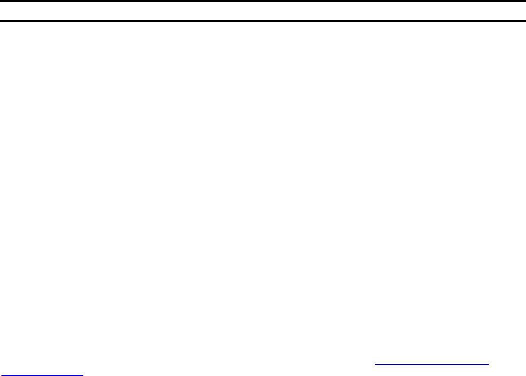
CSO Awareness:

• Placement of informational and

warning signs at CSO outfalls

• Media advis

ories for CSO

events

Public Education:

• Media coverage

• Newsletters/Information book

let

• Educational inserts to water and

sewer bills

• Direct mailers

• CSO project websites

Public Involvement:

• Public meetings

• Funding task force

• Local river committee

• Community leader involvement

Example: Line 11 – Pipe Capacity and Flow Information

• General public telephone

survey

• Focus groups

Successful public participation

occurs when the discussion of CSO

control ha

s involved ratepayers and

users of CSO-impacted

waterbodies.

For more information on public

partici

pation activities, see EPA’s

Combined Sewer Overflows

Guidance for Long-Term Control

CSO 001 CSO 002 CSO 003

a. Type of CSO

hydraulic control

11a

Weir Weir Pump

station

b. CSO hydraulic

control capacity

(MGD)

11b

1.5 1.5 3.0

c. Name of

interceptor or

downstream pipe

11c

South

Street

Interceptor

South

Street

Interceptor

Central

Force

Main

The LTCP-EZ Template: A Planning Tool for CSO Control in Small Communities

Use of Schedules

The LTCP-EZ Template provides an organizational framework for the collection and

presentation of information and analysis that is essential for a draft LTCP. Once

complete, FORM LTCP-EZ (with accompanying schedules) can serve as a draft

LTCP for a small community under appropriate circumstances. Each of the following

three sections on CSO Volume, Evaluation of CSO Controls, and CSO Affordability

include schedules with calculation procedures that are potentially valuable for small

communities. However, although the types of information used in, and generated

by, these schedules is necessary for a draft LTCP, use of these schedules is

optional. Permittees with extremely simple systems, permittees that have already

completed an evaluation of CSO controls, and permittees that have previously

conducted separate analyses may choose not to use these schedules. Under these

circumstances, documentation of the evaluation of CSO control alternatives and

selection of the recommended CSO Control Plan may be provided in another

format.

Plan (EPA 832-B-95-002,

September 1995)

(http://www.epa.gov/npdes/pubs/

owm0272.pdf

Examples of public participation can

also be viewed at the following CSO

project websites:

• City of Lansing, Michigan.

(http://publicservice.cityoflansin

gmi.com/PubEng/cso.jsp)

• City of Manchester, New

Hampshire.

(http://www.manchesternh.gov/

CityGov/DPW/EPD/CSO.html)

• City of St. Joseph, Missouri.

(http://www.ci.st-joseph.mo.us/

publicworks/wpc_cso.cfm

)

• City of Wilmington, Delaware.

(http://www.wilmingtoncso.com/

CSO_home.htm)

Line 12 – Public Participation.

Please check the box on Line 12 to

indicate Schedule 3 – PUBLIC

PARTICIPATION is attached to

FORM L

TCP-EZ. Use Schedule 3 –

PUBLIC PARTICIPATION to

document public participation

activities undertaken (or planned) to

involve the public and stakeholders

in the decision process to evaluate

and select CSO controls.

CSO Volume

The LTCP-EZ Template applies the

“presumption approach” described

in the CSO Control Policy. The

LTCP-EZ Template uses a design

storm approach to identify the

volume of combined sewage that

needs to be stored, treated, or

eliminated to reduce CSOs to no

more than an average of four

overflow events per year. In

accordance with the “presumption

approach” described in the CSO

Control Policy, a program meeting

this criterion is conditionally

presumed to provide an adequate

level of control to meet water

quality-based requirements,

provided that the permitting

authority determines the

presumption is reasonable, based

upon data and analysis provided in

the LTCP.

Use of other criteria under the

“presumption approach” is valid, but

need to be documented separately

(not in Schedule 4 – CSO

VOLUME).

Line 13 – CSO Volume. Please

check the appropriate box on Line

13 to indicate whether Schedule 4 –

CSO VOLUME or separate

documentation is attached to FORM

LTCP-EZ. Schedule 4 – CSO

VOLUME is used to quantify the

volume of combined sewage that

needs to be stored, treated, or

eliminated. This is called the “CSO

volume” throughout the LTCP-EZ

Template. Specific instructions for

completion of Schedule 4 – CSO

VOLUME are provided.

Evaluation of CSO Controls

LTCPs should contain site-specific,

cost-effective CSO controls. Small

communities are expected to

evaluate a simple mix of controls to

assess their ability to provide cost-

effective CSO control. The LTCP-

EZ Template considers the volume

of combined sewage calculated in

Schedule 4 – CSO VOLUME that

needs to be stored, treated, or

eliminated when evaluating

alternatives for CSO controls.

Schedule 5 – CSO CONTROL

provides an evaluation of CSO

control alternatives for the CSO

volume calculated in Schedule 4 –

CSO VOLUME. Specific instructions

for completion of Schedule 5 – CSO

CONTROL are provided. Please

note that Schedule 5 – CSO

CONTROL can be used in an

iterative manner to identify the most

promising CSO control plan with

respect to CSO volume reduction

and cost.

Line 14 – CSO Controls. Please

check the appropriate box on Line

14 to indicate whether Schedule 5 –

CSO CONTROL or separate

documentation is attached to FORM

LTCP-EZ.

Affordability

The CSO Control Policy recognizes

the need to address the relative

importance of environmental and

financial issues when developing an

implementation schedule for CSO

controls. The ability of small

communities to afford CSO control

influences CSO control priorities

and implementation schedule.

Schedule 6 – CSO

AFFORDABILITY provides an

assessment of financial capability in

a two-step process. Step One

involves determination of a

residential indicator to assess the

ability of the resident and the

INSTRUCTIONS: FORM LTCP-EZ

community to afford CSO controls.

Step Two involves determination of

a permittee financial indicator to

assess the financial capability of the

permittee to fund and implement

CSO controls. Information from both

Step One and Step Two is used to

determine affordability.

Line 15 – Affordability. Permittees

are encouraged to assess their

financial capability and the

affordability of the LTCP. Please

check the box in Line 15 if Schedule

6 – CSO AFFORDABILITY is

attached to FORM LTCP-EZ, and

enter the appropriate affordability

burden in Line 15a. Otherwise,

proceed to Line 16.

Line 15a – Affordibility Burden.

Enter the appropriate affordability

burden (low, medium, or high) from

Schedule 6 – CSO

AFFORDABILITY.

Recommended CSO

Control Plan

The LTCP-EZ Template guides

permittees through a series of

analyses and evaluations that form

the basis of a draft LTCP for small

communities. The recommended

CSO controls need to be

summarized so that the permitting

authority and other interested

parties can review them. Line 16 is

used for this purpose.

Line 16 – Recommended CSO

Control Plan. Documentation of the

evaluation of CSO control

alternatives is required (CSO

Control Policy Section II.C.4.).

Permittees that have used Schedule

5 - CSO CONTROL to select CSO

controls should bring the

information from Schedule 5 – CSO

CONTROL forward to Line 16 in

FORM LTCP-EZ. Permittees who

have completed their own

evaluation of CSO alternatives (that

is, permittees that did not use

Schedule 5 – CSO CONTROL)

need to summarize the selected

CSO control on Line16 and attach

the appropriate documentation.

Line 16a – Provide a summary of

the CSO controls selected. This

information can come from the

controls selected on Schedule 5 –

CSO CONTROL, or from other

analyses. Section 3.3.5,

Identification of Control Alternatives,

of EPA’s Combined Sewer

Overflows Guidance for Long-Term

Control Plan document, lists the

various source controls, collection

system controls, and storage and

treatment technologies that may be

viable. This document also

discusses preliminary sizing

considerations, cost/performance

considerations, preliminary siting

issues, and preliminary operating

strategies, all of which should be

discussed on Line 16a of the LTCP-

EZ Template.

Line 16b – Provide a summary of

the cost of CSO controls selected.

Project costs include capital, annual

O&M, and life-cycle costs. Capital

costs should include construction

costs, engineering costs for design

and services during construction,

legal and administrative costs, and

typically a contingency. Annual

O&M costs reflect the annual costs

for labor, utilities, chemicals, spare

parts, and other supplies required to

operate and maintain the facilities

proposed as part of the project. Life-

cycle costs refer to the total capital

and O&M costs projected to be

incurred over the design life of the

project.

At the facilities planning level, cost

curves are usually acceptable for

estimating capital and O&M costs.

When used, cost curves should be

indexed to account for inflation,

using an index such as the

Engineering News Record Cost

Correction Index.

Line 16c – Provide a description of

how the CSO controls selected will

be financed. Discuss self-financing

including fees, bonds, and grants.

Section 4.3, Financing Plan, of

EPA’s Combined Sewer Overflows

Guidance for Long-Term Control

Plan document, states that the

LTCP should identify a specific

capital and annual cost funding

approach. EPA’s guidance on

funding options presents a detailed

description of financing options and

their benefits and limitations, as well

as case studies on different

approaches municipalities took to

fund CSO control projects. It also

includes a summary of capital

funding options, including bonds,

loans, grants, and privatization, as

well as annual funding options for

O&M costs for CSO controls,

annual loan payments, debt service

on bonds, and reserves for future

equipment replacement.

Line 16d –

Describe the proposed

implementation schedule for the

CSO controls selected. The

implementation schedule describes

the planned timeline for

accomplishing all of the program

activities and construction projects

contained in the LTCP. Section

4.5.1.5 of EPA’s Combined Sewer

Overflow Guidance for Permit

Writers document (EPA 832-B-95-

008) summarizes criteria that

should be used in developing

acceptable implementation

schedules, including:

• Phased construction schedules

should consider elimination of

CSOs to sensitive areas and

use impairment.

• Phased schedules should also

include an analysis of financial

capability (see Schedule 6 –

CSO AFFORDABILITY).

• The permittee should evaluate

financing options and data,

including grant and loan

availability, previous and

current sewer user fees and

rate structures, and other viable

funding mechanisms and

sources of funding.

• The schedule should include

milestones for all major

The LTCP-EZ Template: A Planning Tool for CSO Control in Small Communities

implementation activities,

including environmental

reviews, siting of facilities, site

acquisition, and permitting.

• The implementation schedule is

often negotiated with the

permitting authority, and

incorporating the information

listed above in the schedule

provides a good starting point

for schedule negotiations.

The LTCP-EZ Template: A Planning Tool for CSO Control in Small Communities

INSTRUCTIONS: SCHEDULE 4 – CSO VOLUME

Introduction

Understanding the response of the CSS to rainfall is critical for evaluation of the magnitude of CSOs and control needs.

Small CSO communities do not typically have the resources to conduct the detailed monitoring and modeling necessary

to make this determination easily. Schedule 4 – CSO VOLUME of the LTCP-EZ Template provides a simple, conservative

means for assessing CSO control needs. The technical approach contained in Schedule 4 – CSO VOLUME builds upon

the general information and CSS characteristics provided in FORM LTCP-EZ. It rests upon a simple interpretation of the

“presumption approach” described in the CSO Control Policy. Under the “presumption approach”, a CSO community

controlling CSOs to no more than an average of four overflow events per year is presumed to have an adequate level of

control to meet water quality standards.

The volume of combined sewage that needs to be treated, stored, or eliminated is calculated within Schedule 4 – CSO

VOLUME. This is called the “CSO volume.” CSO volume is calculated with a “design storm”, application of the Rational

Method (described below) to determine generated runoff, and use of an empirical equation to estimate excess combined

sewage and conveyance within the CSS. Once construction of controls is completed, it is expected that compliance

monitoring will be used to assess the ability of the controls to reduce CSO frequency to meet the average of four overflow

events per year criterion.

Design Storm for Small Communities

The volume of runoff and combined sewage that occurs due to “design storm” conditions must be controlled to limit the

occurrence of CSOs to an average of four overflow events per year. The LTCP-EZ Template uses two design storm

values, each of which represents a rainfall intensity that, on average, occurs four times per year. These are:

• The statistically-derived one-hour, three-month rainfall. This design storm represents a peak flow condition. It is

reasonably intense, delivers a fairly large volume of rainfall across the CSS, and washes off the “first flush.” In

addition, the one-hour, three-month rainfall facilitates a simple runoff calculation in the Rational Method. The

LTCP must provide control to eliminate the occurrence of CSOs for hourly rainfall up to this intensity.

• The statistically-derived 24-hour, three-month rainfall. This design storm complements the one-hour, three-month

rainfall in the LTCP-EZ Template. The longer 24-hour storm delivers a larger volume of rainfall with the same

three-month return interval. The LTCP must provide control to eliminate the occurrence of CSOs for rainfall up to

this amount over a 24-hour period.

The use of both of these design storms in conjunction with one another ensures that CSO control needs are quantified

based on both rainfall intensity and rainfall volume associated with the return frequency of four times per year.

The Rational Method

The Rational Method is a standard engineering calculation that is widely used to compute peak flows and runoff volume in

small urban watersheds. The Rational Method with a design storm approach is used in the LTCP-EZ Template to quantify

the amount of runoff volume (the “CSO volume”) that needs to be controlled for each CSO outfall and contributing sub-

sewershed area. The Rational Method equation is given as:

Q = kCiA

where:

• Q = runoff (MGD)

• k = conversion factor (acre-inches/hour to MGD)

• C = runoff coefficient (based on land use)

• i = rainfall intensity (in/hr)

• A = sub-sewershed area (acres)

INSTRUCTIONS: SCHEDULE 4—CSO VOLUME

The Rational Method is applied twice within the LTCP-EZ Template: once to determine the peak runoff rate associated

with the one-hour, three-month rainfall, and once to determine the total volume of runoff associated with the 24-hour,

three-month rainfall. When applied properly, the Rational Method is inherently conservative.

Calculation of CSO Volume

CSO volume is calculated within sub-sewersheds at individual CSO hydraulic controls (i.e., weir, orifice) and at the

WWTP. The procedures used to calculate CSO volume are documented in Appendix B. The following operations are

central to these calculations:

• The average dry weather flow rate of sanitary sewage is added to runoff to create a peak hourly flow rate, and is

also used to calculate a total volume of flow over the 24-hour period.

• The ratio of the CSO hydraulic control capacity to the peak flow rate based upon the one-hour, three-month

rainfall determines the fraction of overflow within sub-sewersheds. (Note: Identification of realistic hydraulic

control capacities is an important part of the LTCP-EZ Template. Permittees may need to seek assistance from

qualified professionals to successfully complete this part of the Template. In addition, it is important that

interceptor capacity limitations be taken into account when identifying regulator capacities.)

• The overflow fraction is applied to the total volume of flow associated with the 24-hour, three-month rainfall to

quantify the volume of excess combined sewage at CSO hydraulic controls. This is the “CSO volume” at the CSO

hydraulic control.

• Diversions to the WWTP at CSO hydraulic controls are governed by an empirical relationship based upon the

ratio of the CSO hydraulic control capacity to the peak flow rate and conveyance. The diversions to the WWTP at

CSO hydraulic controls are a component of the peak sewage conveyed to the WWTP.

• The ratio of primary capacity to peak sewage conveyed to the WWTP determines the fraction of combined

sewage untreated at the WWTP. This is the “CSO volume” at the WWTP.

The Schedule 4 – CSO VOLUME results identify the “CSO volum

e,” which is the volume of excess combined sewage that

needs to be stored, treated, or eliminated in order to comply with the “presumption approach.” The results of the

calculations, the excess CSO volumes, are linked to Schedule 5 – CSO CONTROL where control alternatives are

evaluated at the sub-sewershed level and/or at the WWTP.

Summary

The LTCP-EZ Template is designed to provide a very simple assessment of CSO control needs. Prior to entering data

into the LTCP-EZ Template, permittees should collect good information on the characteristics of the CSS, including

reliable information on CSO hydraulic control capacities.

Additional detail and documentation on the approach used to identify overflow, diversion and WWTP overflow fractions is

provided in Appendix B.

The LTCP-EZ Template: A Planning Tool for CSO Control in Small Communities

Sub-Sewershed Area

This section characterizes the

contributing area of each CSO

sub-sewershed area, the

predominant land use, and a runoff

coefficient. These values are

critical inputs to the runoff

calculation developed in this

schedule (the Rational Method).

Schedule 4 – CSO VOLUME is set

up to accommodate up to four sub-

sewersheds. Additional columns

can be added to the schedule as

needed if there are more than four

CSO sub-sewersheds. The

number of sub-sewersheds

evaluated on this schedule needs

to correspond to the system

characterization information

included under Form LTCP-EZ and

the map on Schedule 2 – MAP.

Line 1 – Sub-sewershed area

(acres). Enter the area in acres for

each sub-sewershed in the CSS

(Line 10a on FORM LTCP-EZ. If

you are using the electronic

version of the form, this value will

have been filled in automatically).

Add additional columns if needed.

Line 2 – Principal land use. Enter

the principal land use for each sub-

sewershed area (Line 10b on

FORM LTCP-EZ. If you are using

the electronic version of the form,

this value will have been filled in

automatically).

Line 3 – Sub-sewershed runoff

coefficient. Enter the runoff

coefficient that is most appropriate

for the sub-sewershed on Line 3.

Runoff coefficients represent land

use, soil type, design storm, and

slope conditions. The range of

runoff coefficients associated with

different types of land use is

presented in Table 1. Use the

lower end of the range for flat

slopes or permeable, sandy soils.

Use the higher end of the range for

steep slopes or impermeable soils

such as clay or firmly packed soils.

The higher end of the range can

also be used to add an additional

factor of safety into the calculation.

The runoff coefficient selected

should be representative of the

entire sub-sewershed. Permittees

should consider the distribution of

land use within the sub-sewershed

and develop a weighted runoff

coefficient if necessary. For

example, a sub-sewershed that is

half residential single family

(C=0.40) and half light industrial

(C=0.65) would have a composite

runoff coefficient of C=0.525

[(0.40+0.65)/2].

At a minimum, the runoff

coefficient should be equivalent to

the percent imperviousness for the

sub-sewershed as a decimal

fraction. The percent

imperviousness is the fraction of

each sub-sewershed area that is

covered by impervious surfaces

(such as pavement, rooftops, and

sidewalks) that is directly

connected to the CSS through

catch basins, area drains or roof

leaders.

Runoff

Line 4 Design storm rainfall. The

one-hour, three-month rainfall

intensity (inches per hour) is the

design storm used in the LTCP-EZ

Template to estimate peak runoff

rate. The 24-hour, three-month

rainfall is used to estimate total

volume of runoff generated over a

24-hour period.

Recommended one-hour, three-

month rainfall values by state and

county are provided in Appendix A.

These values are based on

research and products provided by

the Midwest Climate Center

(1992). Values for the Midwestern

states are very specific. Values for

other states in the Northeast have

been approximated based upon

procedures developed by the

Midwest Climate Center. A

statistically derived multiplication

factor of 2.1 is used to convert

these one-hour, three–month

design rainfall conditions into the

24-hour, three–month rainfall

conditions.

Table 1. Runoff Coefficients for Rational Formula

Type of Area (Principal Land Use) Runoff Coefficient (C)

Business – downtown 0.70 -0.95

Business – Neighborhood 0.50-0.70

Residential - Single family 0.30-0.50

Residential – Multi units, detached 0.40-0.75

Residential – Multi units, attached 0.60-0.75

Residential - Suburban 0.25-0.40

Residential – Apartments 0.50-0.70

Industrial - Light 0.50-0.80

Industrial - Heavy 0.60-0.90

Parks, cemeteries 0.10-0.25

Playgrounds 0.20-0.35

Railroad yard 0.20-0.35

Unimproved 0.10-0.30

Source: ASCE (2006)

INSTRUCTIONS: SCHEDULE 4—CSO VOLUME

Site-specific rainfall values or other

design storm intensities may be

used to assess the response of the

CSS to rainfall. However, use of

different rainfall periods may

require a separate analysis outside

of Schedule 4-CSO VOLUME.

Enter the one-hour design storm

rainfall intensity in inches for each

sub-sewershed on Line 4. (Note:

this information is also used in

Schedule 5-CSO CONTROL).

Line 5 – Calculated runoff rate.

Multiply Line 1 by Line 3 and then

this product by Line 4 for each

sub-sewershed area and enter the

result (acre-inches per hour) on

Line 5.

Line 6 – Peak runoff rate in

MGD. Multiply Line 5 by the

conversion factor (k) of 0.6517 and

enter the result for each sub-

sewershed area on Line 6. This is

the one-hour design storm runoff in

MGD.

Dry Weather Flow Within

the CSS

Line 7 – Dry weather flow rate

(MGD).

Enter the average dry

weather flow rate as a rate in MGD

for each sub-sewershed on Line 7.

If dry weather flow is unknown on

a sub-sewershed basis, develop

an estimate supported by 1) direct

measurement of dry weather flow

based on the average of a series

of observations made at different

times of the day; or 2) allocation of

the dry weather flow reported on

the DMR for the WWTP for the

entire sewer service area. Use of

the allocation estimation approach

should take into consideration

characteristics of each sub-

sewershed that influence the rate

of dry weather flow including

population, employment, and

infiltration if known. The sum of dry

weather flow from the CSS plus

the dry weather flow from non-

CSO areas and satellite

communities, if present, should

equal the dry weather flow at the

WWTP.

Line 13 – Volume of runoff (MG).

The volume of runoff for the 24-

hour rainfall is obtained by

multiplying Line 1 by Line 3 and

Line 12 and converting to MG by

applying the conversion factor

0.02215. Enter the product on Line

13.

Peak Wet Weather Flow

Line 8 – Peak flow rate (MGD).

The peak flow rate is the sum of

the peak runoff rate and dry

weather flow in MGD. Add Lines 6

and 7 and enter the sum for each

sub-sewershed area on Line 8.

Line 14 – Volume of dry weather

flow (MG). This is the total dry

weather flow in MG for the 24-hour

design rainfall period. It is

calculated by multiplying the dry

weather flow rate in MGD on line 7

by 24 hours. Enter this value on

Line 14.

Overflow

Line 9 – CSO hydraulic control

capacity (MGD). CSO hydraulic

control capacity is the maximum

flow that the sub-sewershed area

sewer can deliver to the interceptor

sewer. Enter the CSO hydraulic

control capacity in MGD for each

CSO sub-sewershed area on Line

9 (Line 11b on FORM LTCP-EZ. If

you are using the electronic

version of the form, this value will

have been filled in automatically).

Line 15 – Total volume of flow

(MG). This is the total volume of

flow in MG within each sub-

sewershed for the 24-hour design

rainfall period. Add Lines 13 and

14 and enter the sum on Line 15.

Line 16 – Volume of excess

combined sewage at individual

CSO hydraulic controls during

24-hour rainfall period. This is

also the “CSO volume” at the CSO

hydraulic control and is the

combined sewage that exceeds

the diversion capacity determined

by the CSO hydraulic control in

each sub-sewershed. Multiply Line

11 by Line 15 and enter the

product on Line 16.

Line 10 – Ratio of CSO hydraulic

control capacity to peak flow

rate. Enter 1.0 on Line 10 if Line 9

is greater than Line 8. Otherwise,

divide Line 9 by Line 8 and enter

the quotient (result) on Line 10.

Line 11 – Overflow fraction of

combined sewage. This is the

overflow fraction of combined

sewage within the sub-sewershed.

It is based on the ratio of CSO

hydraulic control capacity to peak

flow rate. Take the square of (1

minus the value on Line 10) and

enter it on Line 11. For example, if

the ratio of CSO hydraulic control

capacity to peak flow rate on Line

10 is 0.15, the overflow fraction is

(1-0.15)

, or 0.7225.

Diversion

Line 17 – Diversion fraction of

combined sewage. This is the

fraction of runoff within each

subsewershed that is collected and

diverted to the WWTP over the 24-

hour design storm period. The

diversion fraction is based on the

ratio of CSO hydraulic control

capacity to peak flow rate and

conveyance. Determine the

diversion fraction of combined

sewage from Line 10 using Table

2, and enter on Line 17.

Line 12 – 24-hour rainfall.

Multiply Line 4 by 2.1 to obtain the

24-hour design rainfall and enter

the product on Line 12.

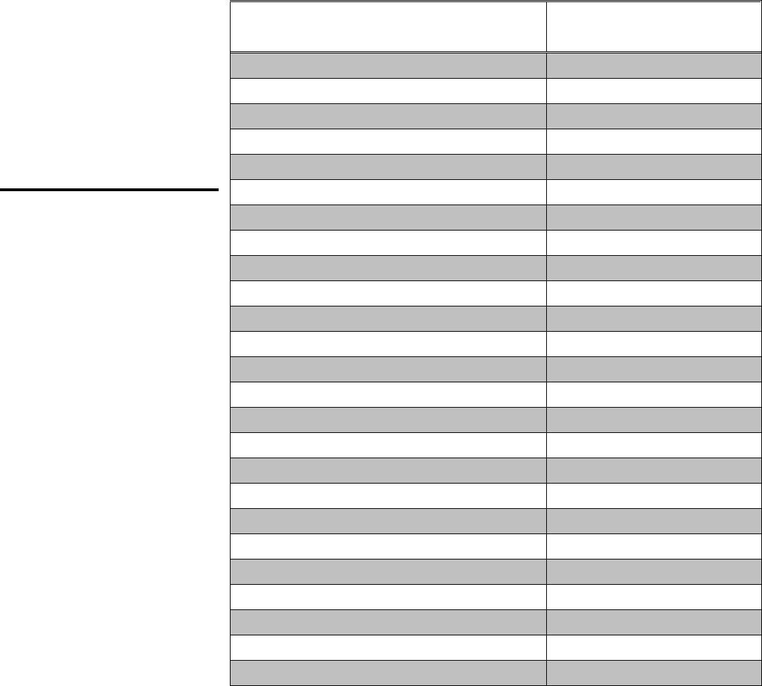
The LTCP-EZ Template: A Planning Tool for CSO Control in Small Communities

Line 18 – Volume of runoff

diverted to WWTP. This is the

volume of runoff within each sub-

sewershed that is collected and

diverted to the WWTP over the

24-hour design storm period.

Multiply Line 13 by Line 17 and

enter the product on Line 18.

Line 19 – Total volume of

combined sewage conveyed to

WWTP during 24-hour rainfall

period (MG). Add Lines 14 and

18 and enter the sum on Line 19.

Conveyance

Line 20 – Peak rate of collected

combined sewage diverted to

the WWTP within sub-

sewersheds. Identify the smaller

of Line 8 and Line 9 within each

sub-sewershed and enter the

peak rate in MGD on Line 20.

Line 21 – Peak rate of

combined sewage conveyed to

WWTP (MGD). This peak rate

represents the sum of the peak

rates of collected combined

sewage diverted to the WWTP

from individual sub-sewersheds in

MGD. Add up sub-sewershed

values on Line 20 and enter on

Line 21.

Line 22 – Peak rate of sewage

from non-CSO areas (MGD).

Non-CSO areas can be affected

by wet weather conditions due to

I/I. the degree to which the peak

rate of sewage in non-CSO areas

is higher than the average dry

weather flow rate depends on

site-specific conditions. Direct

measurement of the peak rate of

sewage during wet weather is the

Table 2. Diversion Fraction of Combined Sewage from 24-Hour Storm

Ratio of CSO Hydraulic Control Capacity to

Peak Flow Rate

Diversion Fraction

0.01 to 0.02 0.04

0.02 to 0.03 0.06

0.03 to 0.04 0.09

0.04 to 0.05 0.11

0.05 to 0.06 0.14

0.06 to 0.07 0.16

0.07 to 0.08 0.19

0.08 to 0.09 0.21

0.09 to 0.10 0.24

0.10 to 0.12 0.28

0.12 to 0.14 0.33

0.14 to 0.16 0.38

0.16 to 0.18 0.42

0.18 to 0.20 0.47

0.20 to 0.24 0.54

0.24 to 0.28 0.62

0.28 to 0.32 0.68

0.32 to 0.36 0.72

0.36 to 0.40 0.76

0.41 to 0.50 0.81

0.51 to 0.60 0.87

0.61 to 0.70 0.91

0.71 to 0.80 0.95

0.81 to 0.90 0.98

0.91 to 1.0 0.99

INSTRUCTIONS: SCHEDULE 4—CSO VOLUME

best approach for determining this

rate. Estimation based on flow

measured at the WWTP and local

knowledge of the distribution of

flow in the service area provides

another approach. Peaking factors

can also be used to adjust the

average dry weather flow upward.

Newer “tight” sewer systems may

have peaking factors between 1.0

and 1.5. Older, leakier systems

may have peaking factors between

1.5 and 3.0, or even higher. Enter

the peak rate of sewage conveyed

to the WWTP from non-CSO areas

in the community in MGD on Line

22.

Line 23 – Peak rate of sewage

from satellite communities

(MGD). Satellite communities can

be affected by wet weather

conditions due to I/I. the degree to

which the peak rate of sewage in

satellite communities is higher than

the average dry weather flow rate

depends on site-specific

conditions. Direct measurement of

the peak rate of sewage during wet

weather is the best approach for

determining this rate. Estimation

based on flow measured at the

WWTP and local knowledge of the

distribution of flow in the service

area provides another approach.

Peaking factors can also be used

to adjust the average dry weather

flow upward. Newer “tight” sewer

systems may have peaking factors

between 1.0 and 1.5. Older, leakier

systems may have peaking factors

between 1.5 and 3.0, or even

higher. The maximum rate of flow

from capacity agreements may

also be used and may be more

appropriate than measurements or

estimates. Enter the peak rate of

sewage conveyed to the WWTP

from satellite communities in MGD

on Line 23.

Line 24 – Peak rate of sewage

conveyed to the WWTP (MGD).

This is the peak rate of sewage

flow in MGD received at the

WWTP from the CSS and adjacent

non-CSO areas in the community

and satellite communities. Add

Lines 21, 22 and 23 and enter the

sum on Line 24.

Treatment

Line 25 – Primary treatment

capacity

(MGD). Enter the primary

treatment capacity in MGD on Line

25 (Line 4a on FORM LTCP-EZ. If

you are using the electronic

version of the form, this value will

have been filled in automatically).

Use of primary treatment capacity

for CSO control is a viable option

where approval of the regulatory

agency has been obtained. The

CSO Control Policy indicates that

combined sewer flows remaining

after implementation of the NMCs

and within the criteria under the

“presumption approach” at a

minimum should receive:

• Primary clarification (removal

of floatables and settleable

solids may be achieved by any

combination of treatment

technologies or methods that

are shown to be equivalent to

primary clarification);

• Solids and floatables disposal;

and

• Disinfection of effluent, if

necessary, to meet WQS,

protect designated uses and

protect human health,

including removal of harmful

disinfection residuals, where

necessary.

The Combined Sewer Overflows

Guidance for Long

-Term Control

Plan document, Section 3.3.3.5,

Utilization of POTW Capacity and

CSO-Related Bypass, addresses

the specific case where existing

primary treatment capacity

exceeds secondary treatment

capacity and it is not possible to

utilize the full primary treatment

capacity without overloading the

secondary facilities. For such

cases, the CSO Control Policy

states that at the request of the

municipality, EPA may allow an

NPDES permit “…to authorize a

CSO-related bypass of the

secondary treatment portion of the

POTW treatment plant for

combined sewer overflows in

certain identified circumstances”

(II.C.7). Under this provision, flows

to the POTW within the capacity of

primary treatment facilities but in

excess of the capacity of

secondary treatment facilities may

be diverted around the secondary

facilities provided that “…all wet

weather flows passing the

headworks of the POTW treatment

plant will receive at least primary

clarification and solids and

floatables removal and disposal,

and disinfection, where necessary,

and any other treatment that can

be reasonably provided” (II.C.7).

In addition, the CSO-related

bypass should not cause

exceedance of WQS.

Line 26 – Ratio of primary

treatment capacity to peak rate

of sewage conveyed to WWTP.

Enter 1.0 on Line 26 if Line 25 is

greater than Line 24. Otherwise,

divide Line 25 by Line 24 and enter

the quotient (result) on Line 26.

Line 27 –Fraction of combined

sewage untreated at WWTP. This

is the fraction of sewage delivered

to the WWTP during the 24-hour

rainfall period that does not

received primary treatment. It is

based on the ratio of primary

treatment capacity to peak rate of

sewage conveyed to the WWTP.

Take the square of (1 minus the

value on Line 26) and enter it on

Line 27. For example, if the ratio of

primary treatment capacity to peak

rate of sewage conveyed to the

WWTP on Line 26 is 0.80, the

overflow fraction is (1-0.80)

, or

0.04.

The LTCP-EZ Template: A Planning Tool for CSO Control in Small Communities

Line 28 – Sum of combined

sewage conveyed to WWTP

during 24-hour rainfall period

(MG). Add up the sub-sewershed

values in MG on Line 19 and enter

on Line 28.

Line 29 – Dry weather flow from

the non-CSO area (MGD). Enter

the dry weather flow rate from the

non-CSO area in MGD on Line 29.

If dry weather flow for the non-

CSO area is unknown, develop an

estimate supported by 1) direct

measurement of dry weather flow

based on the average of a series

of observations made at different

times of the day; or 2) allocation of

the dry weather flow reported on

the DMR for the WWTP for the

entire sewer service area.

Line 30- Volume of sewage from

non-CSO areas during 24-hour

rainfall period (MG). The volume

of sewage from non-CSO areas

during the 24-hour rainfall period is

likely to be higher than the average

dry weather flow rate (Line 29)

because of I/I, but less than the

peak rate of sewage (Line 22).

Typical daily wet weather volumes

should be used if measurements

are available. Alternatively, an

estimate based on the peak rate of

sewage (Line 22) and the dry

weather flow rate (Line 29) can be

used. Under this approach, it is

assumed that flow to the WWTP

from the non-CSO area over the

course of the 24-hour rainfall

period has a triangular shape. The

volume is calculated by adding

one-half the difference between

Line 22 and 29 and adding this

value to the dry weather flow rate.

Subtract Line 29 from Line 22,

divide by 2, add the remainder to

Line 29, and enter this value as a

volume in MG on Line 30.

Line 31 – Dry weather flow from

the satellite communities (MGD).

Enter the dry weather flow rate

from the satellite communities in

MGD on Line 29. If dry weather

flow for the satellite communities is

unknown, develop an estimate

supported by 1) direct

measurement of dry weather flow

based on the average of a series

of observations made at different

times of the day; or 2) allocation of

the dry weather flow reported on

the DMR for the WWTP for the

entire sewer service area.

Line 32- Volume of sewage from

satellite communities during 24-

hour rainfall period (MG). The

volume of sewage from satellite

communities during the 24-hour

rainfall period is likely to be higher

than the average dry weather flow

rate (Line 31) because of I/I, but

less than the peak rate of sewage

(Line 23). Typical daily wet

weather volumes should be used if

measurements are available.

Alternatively, an estimate based on

the peak rate of sewage (Line 23)

and the dry weather flow rate (Line

31) can be used. Under this

approach, it is assumed that flow

to the WWTP from the satellite

communities over the course of the

24-hour rainfall period has a

triangular shape. The volume is

calculated by adding one-half the

difference between Line 23 and 31

and adding this value to the dry

weather flow rate. Subtract Line 31

from Line 23, divide by 2, add the

remainder to Line 31, and enter

this value as a volume in MG on

Line 32.

Line 33 – Total volume of

sewage during 24-hour rainfall

event (MG). Add Lines 28, 30 and

32 and enter the volume in MG on

Line 33.

Line 34 – Volume of combined

sewage untreated at WWTP

(MG). This is also the “CSO

volume” at the WWTP. Enter 0.0

on Line 34 if Line 25 is greater

than Line 24. Otherwise, multiply

Line 31 by Line 27 and enter the

volume in MG on Line 34.

CSO Volume

The CSO volume that needs to be

stored, treated or eliminated is

calculated in SCHEDULE 4- CSO

Volume. These CSO volumes are

identified within individual sub-

sewersheds at CSO hydraulic

controls, and at the WWTP.

Line 35 – Volume of combined

sewage overflows at CSO

outfalls (MG). This represents the

volume of excess combined

sewage in MG that is discharged

at CSO outfalls. Sum all sub-

sewershed volumes in MG on Line

16 and enter on Line 35.

Line 36 – Volume of combined

sewage overflow at WWTP (MG).

This represents the volume of

excess combined sewage in MG

that is collected and conveyed to

the WWTP that does not receive at

least primary treatment. Enter the

value on Line 34 on Line 36.

The LTCP-EZ Template: A Planning Tool for CSO Control in Small Communities

INSTRUCTIONS: SCHEDULE 5 – CSO CONTROL

The calculation in Schedule 4 – CSO VOLUME quantifies the volume of combi

ned sewage generated by a storm that

occurs no more than four times per year (once every three months). This is the volume of combined sewage that needs

to be stored, treated, or eliminated under the “presumption approach” so that there are no more than an average of four

overflow events per year. The calculation leads the permittee to identify the rate and volume of combined sewage

conveyed to the WWTP. It also identifies the rate and volume of combined sewage at sub-sewershed outfalls governed by

CSO hydraulic controls. This schedule is intended to help the permittee evaluate the ability of a limited number, but widely

used, set of CSO controls to store, treat, or eliminate excess combined sewage.

The permittee is expected to develop a simple LTCP based upon CSS characterization, the hydraulic response of the

CSS to rainfall established in Schedule 4 – CSO VOLUME, information presented on CSO controls, and an understanding

of local conditions and circumstances. Schedule 5 – CSO CONTROL provides a simple approach to organize and

evaluate control needs, performance, and costs. Small communities can use this schedule in an iterative manner to

identify the mix of CSO controls needed.

Four general methods for CSO control are considered in this schedule. They are:

• Conveyance and treatment at the WWTP

• Inflow reduction for residential properties

• Sewer separation

• Off-line storage

It is recommended that permittees evaluate these con

trols in the order presented. Use of more than one CSO control in a

LTCP is common. Use of other controls not described herein is valid, but would have to be documented separately in a

similar effort to what is presented in this schedule.

Schedule 5 – CSO CONTROL should be used in an iterative manner in order to identify the most appropriate mix of CSO

controls with respect to CSO reduction and cost. The volumes of combined sewage at CSO outfalls and at the WWTP that

need to be controlled (Lines 33 and 34 on Schedule 4 – CSO VOLUME) serve as the reduction targets for this schedule.

Conveyance and Treatment at the WWTP

Maximization of treatment at the existing WWTP is emphasized in the CSO Control Policy, and it is an important feature of

many LTCPs. In some CSO communities, the ability to convey combined sewage to the WWTP exceeds the primary

capacity of the WWTP. The presence of this condition is assessed in Schedule 4 – CSO VOLUME, and the use of

additional storage or treatment capacity at the WWTP is included in this schedule. The schedule is not set up to evaluate

the opposite situation, where the WWTP has excess primary treatment capacity. Permittees with this situation can

potentially make use of available primary treatment capacity at the WWTP by adjusting CSO hydraulic controls, increasing

interceptor conveyance capacity, or increasing pumping capacity. This analysis needs to be documented separately and

attached to this schedule.

Inflow Reduction

Inflow reduction is a widely used CSO control practice centered on removal of direct sources of storm water connected to

the CSS. Roof leader redirection and down spout disconnection are the only inflow reduction measure considered in this

schedule. This practice has been implemented successfully in many CSO communities. It is applicable in small CSO

communities where lawns and green space are abundant and are underlain with permeable soils.

Citywide surveys are often necessary to determine the extent of roof leader connections to the CSS. Inflow control

through roof leader disconnection can be voluntary or mandatory. The best results are achieved where disconnection

programs are widely implemented in a community. Some communities have offered financial incentives to property

owners to encourage participation, while others have linked roof leader disconnection efforts with efforts to redirect area

drains, foundation drains, and sump pumps. Roof leader and down spout disconnection programs are most successful

INSTRUCTIONS: SCHEDULE 5—CSO CONTROL

when they are accompanied by an educational component so that homeowners fully understand the importance of

keeping flows from roof leaders and downspouts out of the collection system. In addition, most successful programs

include continued municipal surveys or inspections to ensure that the program is working. This evaluation of CSO control

alternatives is limited to roof leaders and down spouts from residential buildings because the design storm calculation

lends itself to control of the volume of rain that falls on a rooftop. The analysis of other forms of inflow reduction such as

basement sump pump redirection and low impact development practices is not possible in this schedule, but can be

documented separately and appended to this schedule.

Note

: the LTCP-EZ Template contains calculations for inflow reduction, which is the component of I/I that is associated

with wet weather and directly-connected impervious area. Infiltration is accounted for in the dry weather flow entered on

Line 7 of Schedule 4 – CSO VOLUME. If communities wish to examine infiltration reduction and its effect on reducing

CSO volumes, they can adjust the dry weather flow rate to incorporate infiltration reduction and re-examine the results of

the Schedule 4 – CSO VOLUME calculations.

Sewer Separation

Sewer separation is the practice of replacing the single pipe system of a CSS with separate pipes for sanitary and storm

water flows. Sewer separation is highly effective and widely used. However, it can be expensive relative to other CSO

controls. While sewer separation can be implemented on a broad basis across an entire CSS, it is most often

implemented in selective portions of the CSS where localized circumstances make it less disruptive and more economical.

It should also be noted that while sewer separation can help to mitigate CSO issues, it can increase the burden on the

storm sewer system.

Off-Line Storage

“Off-line storage” is a phrase used to describe facilities that store combined sewage in added tanks, basins, tunnels or

other structures. During dry weather, wastewater is passed around, not through, off-line storage facilities. During wet

weather, combined sewage flows are diverted from the CSS to the off-line facility by gravity drainage or with pumps. The

stored combined sewage is temporarily detained in the storage facility and returned to the CSS once conveyance and

treatment capacity become available.

Off-line storage facilities can be expensive relative to other CSO controls. Near surface storage facilities probably have

the most utility because space may be more readily available in small communities, and design, construction and O&M

costs are less than the cost of deep underground tanks and tunnels.

Cost of CSO Control

Generalized cost information for CSO controls is provided. Background information or the derivation of this cost

information is contained in Appendix C. Permittees should realize that CSO control costs are highly variable and

dependent on site-specific conditions. Use of actual or local cost data is always preferable where it is available.

Permittees should verify the appropriateness of default cost values where they are used. Permittees should also note that

cost estimates are for the construction of facilities. Additional operational costs and treatment costs are not expressly

included in cost estimates for controls where primary capacity is added or where combined sewage is temporarily stored

on-site at the WWTP or off-line and released for treatment following the rainfall event.

Summary

More information can be found in EPA’s CSO control technology description at

http://www.epa.gov/npdes/pubs/csossoRTC2004_AppendixL.pdf

The LTCP-EZ Template: A Planning Tool for CSO Control in Small Communities

Conveyance and Treatment

at the WWTP

This section of Schedule 5 – CSO

CONTROL considers conveyance

and treatment of combined sewage

at the WWTP. Additional treatment

or storage can be added at the

WWTP if the ability of the CSS to

convey combined sewage to the

WWTP exceeds primary capacity.

Conversely, excess primary

capacity at the WWTP provides an

opportunity to maximize flow of

combined sewage to the WWTP for

treatment.

Skip to Line 10 if you are not

evaluating control alternatives at the

WWTP.

Line 1 – Peak rate of sewage

conveyed to WWTP (MGD). Enter

the peak rate of sewage conveyed

to the WWTP in MGD on Line 1

(Line 24 on Schedule 4 – CSO

VOLUME. If you are using the

electronic version of the form, this

value will have been filled in

automatically).

Line 2 – Primary treatment

capacity (MGD). Enter the primary

treatment capacity in MGD on Line

2 (Line 25 of Schedule 4 – CSO

VOLUME. If you are using the

electronic version of the form, this

value will have been filled in

automatically).

Line 3 – Difference between

primary treatment capacity and

peak rate of sewage conveyed to

WWTP (MGD). Enter the combined

sewage untreated at the WWTP in

MGD (Line 32 on Schedule 4 –

CSO VOLUME. If you are using the

electronic version of the form, this

value will have been filled in

automatically).

Untreated combined sewage at the

WWTP can be controlled by adding

additional treatment capacity (Line

4) or by adding storage (Line 7) to

allow collected combined sewage to

be retained temporarily until

treatment capacity becomes

available following the rainfall event.

Permittees can estimate costs for

both options and determine which is

most appropriate for their facility.

Note

: If Line 2 is greater than Line

1, the difference represents primary

treatment capacity that may be

available for treatment of combined

sewage. Maximization of flow to the

WWTP should be pursued under

these circumstances. This could be

done iteratively in Schedule 4 –

CSO VOLUME by adjusting

hydraulic control capacities, or

assessed in worksheets to

supplement the LTCP-EZ Template.

Line 4 – Additional primary

treatment capacity required

(MGD). Additional primary treatment

capacity may be added to the

system in order to treat the

combined flows that reach the

WWTP during wet weather. Line 3

represents the minimal additional

primary treatment capacity that will

be required to treat these flows.

Permittees may either enter the

value from Line 3 on Line 4, or they

may enter a larger number if they

want to increase primary treatment

capacity even further.

Line 5 – Unit cost of primary

treatment per MGD. The unit cost

of primary treatment varies greatly.

Enter a cost that reflects local site-

specific conditions, or use the

default value of $2,000,000 per

MGD.

Line 6 – Estimated cost of new

primary treatment capacity at

WWTP. Multiply the unit cost on

Line 5 by the additional capacity

required on Line 4.

Line 7 – Volume of storage

required at WWTP (MG). The

volume of storage required is

determined by converting the flow

rate in MGD on Line 3 to a volume

in MG by multiplying Line 3 by 24

hours. Enter this value on Line 7.

Line 8 – Unit cost of additional

storage at WWTP. The unit cost of

storage varies greatly. Enter a cost

that reflects local site-specific

conditions, or use the default value

of $1,000,000 per MG.

Line 9 – Estimated cost for

storage at WWTP. Multiply the

additional storage volume required

on Line 7 by the unit cost on Line 8.

Inflow Reduction –

Residential

Inflow reduction refers to techniques

used to reduce the amount of storm

water that enters a CSS. Roof

leader redirection and downspout

disconnection are featured in the

LTCP-EZ Template because they

have been used successfully by

many CSO communities. Roof

leader redirection and downspout

disconnection are most applicable

in urban neighborhoods where roof

leaders and downspouts on

residential dwellings currently

draining to the CSS are redirected

to lawns and yards. Redirected flow

then infiltrates into the soil.

Line 10 – 24-hour design rainfall

(inches). Enter the 1-hour design

rainfall in inches on Line 10 (Line 12

on Schedule 4—CSO VOLUME. If

you are using the electronic version

of the form, this value will have

been filled in automatically).

Line 11 – Number of residential

dwellings participating in inflow

reduction. Enter the number of

residential dwellings within each

sub-sewershed that are considered

for roof leader redirection as an

inflow reduction measure.

Permittees should consider

reducing this number slightly to

account for implementation

inefficiency.

INSTRUCTIONS: SCHEDULE 5—CSO CONTROL

Line 12 – Average roof area of

residential dwellings (Sq. Ft.).

The roof area of residential

dwellings varies greatly between the

range of 1,000 and 4,000 square

feet. Roof areas tend to be smaller

in highly urban areas with town

houses and row houses, and larger

in suburban or small town settings.

Enter a value that is characteristic

of dwellings in the sub-

sewershed(s) or use a default value

of 1,200 square feet. This can

sometimes be estimated from GIS

or from real estate aerial

photographs.

Line 13 – Runoff to CSS

eliminated due to inflow

reduction (Gal.). Multiply Lines 10,

11 and 12. Multiply the product by

0.6234 to convert to gallons.

Line 14 – Volume reduction (MG).

Enter the volume reduction

achieved through inflow reduction.

Divide Line 13 by one million.

Line 15 – Unit cost per dwelling

unit for residential inflow

reduction. The unit cost of roof

leader redirection varies depending

on incentives and homeowner

investment. Enter a cost that

reflects local site-specific

conditions, or use the default value

of $250 per dwelling unit.

Line 16 – Estimated cost of

residential inflow reduction.

Multiply the number of dwellings

considered for roof leader

redirection on Line 11 by the unit

cost per dwelling on Line 15.

Sewer Separation

Sewer separation is the practice of

separating the single pipe system of

a CSS into separate pipe systems

for sanitary and storm water flows.

Sewer separation is widely used as

a CSO control. It is often applied

opportunistically in small sub-areas

to minimize disruption. Some small

communities also invest in sewer

separation on a system-wide basis.

Line 17 – Sub-sewershed area to

be separated (acres). Enter the

area to be separated in each sub-

sewershed.

Line 18 – Runoff coefficient of

area to be separated. Enter the

runoff coefficient entered on Line 3

on Schedule 4 – CSO VOLUME.

Line 19 – Runoff to CSS

eliminated due to sewer

separation (Gal.). Multiply Lines

10, 17 and 18. Multiply the product

by 27,156 to convert to gallons.

Line 20 – Volume reduction (MG).

Enter the volume reduction

achieved through sewer separation.

Divide Line 19 by one million.

Line 21 – Unit cost of sewer

separation per acre. The unit cost

of sewer separation is highly

variable. Estimates range from less

than $10,000 to over $200,000 per

acre. Enter a cost that reflects local

site-specific conditions, or use the

default value of $40,000 per acre.

Line 22 – Estimated cost of sewer

separation.

Multiply the number of

acres to be separated on Line 17 by

the unit cost on Line 21 and enter

on Line 22.

Off-Line Storage

The use of storage facilities to store

and attenuate peak combined

sewage flows is widely used as a

CSO control. Off-line storage is the

term used to describe facilities that

store excess combined sewage in

tanks, basins, tunnels, or other

structures located adjacent to the

CSS.

Line 23 – Volume reduction to be

achieved with storage (MG). Enter

the proposed volume of storage in

each sub-sewershed. This can be

established as the original volume

of excess combined sewage at

individual CSO hydraulic controls

(Line 16 on Schedule 4 – CSO

VOLUME) minus reductions

achieved through inflow reduction

and sewer separation.

Line 24 – Unit cost per MG of

storage. The unit cost of off-line

storage is highly variable and

ranges from less than $100,000 per

MG to several million dollars per

MG. Enter a cost that reflects local

site-specific conditions, or use the

default value of $1,000,000 per MG.

Line 25 – Estimated cost of

storage. Multiply Line 23 by Line

24.

Summary of Controls and

Costs

The final CSO control alternatives

selected on this schedule (and on

supporting analysis if used)

represent the CSO controls

proposed for the draft LTCP. The

level of CSO control proposed must

be consistent with the CSO volumes

determined to require control on

Line 23 and 24 of Schedule 4 –

CSO VOLUME.

Complete the following summary of

recommended CSO controls and

costs below and on FORM LTCP-

EZ.

Line 26 – Volume reduction from

CSO controls in sub-sewersheds

(MG). Add Lines 14, 20 and 23.

Line 27– Cost of CSO controls in

sub-sewersheds. Add Lines 16, 22

and 25.

Line 28 – Total volume reduction

in sub-sewersheds (MG). Add up

volumes across Line 26.

Line 29 – Total cost of CSO

controls in sub-sewersheds. Add

up costs across Line 27.

The LTCP-EZ Template: A Planning Tool for CSO Control in Small Communities

Line 30 – Total cost of additional

treatment or storage at WWTP.

Select cost on Line 6 or Line 9.

Enter 0.0 if no additional control is

planned at the WWTP.

The LTCP-EZ Template: A Planning Tool for CSO Control in Small Communities

INSTRUCTIONS: SCHEDULE 6 – CSO AFFORDABILITY

The CSO Control Policy recognizes the need to ad

dress the relative importance of environmental and financial issues

when developing an implementation schedule for CSO controls. The ability of small communities to afford CSO control

influences control priorities and the implementation schedule. Schedule 6 – CSO AFFORDABILITY uses EPA’s

affordability analysis approach to develop a financial capability indicator for the community. This financial capability

indicator is

not to be interpreted as an indicator of whether or not communities can afford CSO controls; rather, the

affordability analysis is used as part of the planning process to determine the potential burden on the community for

implementing the controls over a specific schedule. Thus, one of the primary uses of the affordability analysis is in the

negotiation of the CSO control implementation schedule.

The affordability analysis standardiz

es the determination of financial burden by using standard “big-picture” measures of a

community’s financial capability (e.g., property tax rates, median household incomes, bond ratings, etc.) so that it can be

compared across municipalities without regard to a community’s individual method for funding wastewater and collection

system projects. Once the overall financial capability is determined for a community, it can be used in discussions with

regulators to determine a realistic schedule for implementing CSO controls that takes into account the financial burden to

the community in implementing those controls.

This Schedule presents a two-phase approach to assessing a permittee’s financial capability. The first phase identifies the

combined impact of wastewater and CSO control costs on individual households. The second phase examines the debt,

socioeconomic, and financial conditions of a permittee. The results of the two-phase analysis are combined in a Financial

Capability Matrix. As discussed above, permittees and the water quality standards and NPDES authorities can then use

the matrix to assess the financial burden of the CSO control costs and establish a reasonable schedule to implement the

CSO controls.

Phase I determines a Residential Indicator. This indicator is the permittee’s average costs per household (CPH) for

wastewater treatment (WWT) and CSO controls as a percentage of the local median household income (MHI). It reflects

the residential share of current and planned WWT and CSO control needs to meet the requirements of the Clean Water

Act. A value for this indicator characterizes whether costs will impose a “low’, “mid-range”, or “high” financial impact on

residential users.

Phase II develops the permittee’s Financial Capability Indicators. Six indicators are used to evaluate the debt,

socioeconomic and financial conditions that affect a permittee’s financial capability to implement the CSO controls. These

indicators serve as the basis for a second phase analysis that characterizes the permittee’s financial capability as “weak”,

“mid-range”, or “strong”. Schedule 6 – CSO AFFORDABILITY is based on EPA’s Combined Sewer Overflows–Guidance

for Financial Capability Assessment and Schedule Development. This guidance is located at

http://www.epa.gov/npdes/pubs/csofc.pdf

INSTRUCTIONS: SCHEDULE 6—CSO AFFORDABILITY

Phase I Residential

Indicator

In Phase I of the analysis of the

permittee’s financial capability, a

Residential Indicator is calculated.

The Residential Indicator

measures the financial impact of

the current and proposed

wastewater treatment (WWT) and

CSO controls on residential users.

Development of this indicator

starts with the determination of the

current and proposed WWT and

CSO control costs per household

(CPH). Next, the service area's

CPH estimate and the median

household income (MHI) are used

to calculate the Residential

Indicator. Finally, the Residential

Indicator is compared to

established financial impact ranges

to determine whether CSO

controls will produce a possible

high, mid-range or low financial

impact on the permittee's

residential users.

The first step in developing the

CPH is to determine the

permittee's total WWT and CSO

costs by adding together the

current costs for existing

wastewater treatment operations

and the projected costs for any

proposed WWT and CSO controls.

The next step is to calculate the

residential share of the total WWT

and CSO costs. The final step is to

calculate the CPH by dividing the

residential share of total WWT and

CSO costs by the number of

households in the permittee's total

wastewater service area.

The permittee's latest financial

reports should be used to develop

the current wastewater treatment

operations costs. In order to

comply with accounting

requirements, most permittees

develop a combined statement of

revenues, expenses, and changes

in fund balance. These reports

should be available directly from

the accounting or financial

departments in the permittee’s

community, or, in some states,

from central records kept by the

state auditor or other state offices

(many states conduct audits and

generate financial reports - i.e.,

balance sheet, statement of

revenues, expenses, changes in

fund balances, and statement of

cash flows, for each permittee.)

Projected costs and the number of

households in the wastewater

service area should be available

through planning documents.

The Bureau of Labor Statistics

website at

http://factfinder.census.gov/home/

saff/main.html?_lang=en

has data

that can be used to estimate the

number of households in a specific

service area. The Consumer Price

Index rate (CPI) is used in several

calculations. The value used

should be the average rate for the

previous five years. The CPI is

available through the Bureau of

Labor Statistics website at

http://www.bls.gov/cpi/

The first step in developing the

Residential Indicator is to

determine the Cost Per Household

of total WWT and CSO Costs. In

order to do this, permittees must

first calculate current WWT and

CSO costs, and then projected

costs of future WWT and CSO

treatment. These steps are

completed in Lines 1-17 below.

Current Costs

Current WWT costs are defined as

current annual wastewater

operating and maintenance

expenses (excluding depreciation)

plus current annual debt service

(principal and interest). This is a

fair representation of cash

expenses for current wastewater

treatment operations (expenses for

funded depreciation, capital

replacement funds, or other types

of capital reserve funds are not

included in current WWT costs,

because they represent a type of

savings account rather than an

actual operation and maintenance

expense).

Line 1 – Annual operations and

maintenance expenses

(excluding depreciation). Enter

the annual operation and

maintenance costs -including all

significant cost categories, such as

labor, chemicals,

utilities, administration, and

equipment replacement. Do not

include depreciation.

Line 2 – Annual debt service

(principal and interest). Enter the

annual debt service paid on WWT

debts.

Line 3 – Current costs. Add

together the annual operations and

maintenance expenses from Line 1

and the annual debt service from

Line 2 and enter on Line 3.

Projected Costs (Current

Dollars)

Estimates of projected costs are

made for proposed WWT projects

and for CSO controls. Any

concerns about including specific

proposed WWT projects or CSO

controls in the projected costs, or

the length of the planning period,

should be discussed with the

appropriate NPDES permitting and

enforcement authorities. These

costs should include projected

operation and maintenance

expenses plus projected debt

service costs for any proposed

WWT and CSO controls. The

residential or household costs

(Lines 12 -17) exclude the portion

of expenses attributable to

commercial, governmental and

industrial wastewater discharges.

These costs are adjusted to

current dollars (i.e., deflated).

The LTCP-EZ Template: A Planning Tool for CSO Control in Small Communities

Line 4 – Projected annual

operations and maintenance

expenses (excluding

depreciation). Enter the projected

annual WWT and costs for new

CSO-related facilities.

Line 5 – Present value

adjustment factor. The present

value adjustment factor may be

calculated using the formula

presented below. The formula

converts projected costs to current

dollars using the average annual

national Consumer Price Index

(CPI) inflation rate (available from

the Bureau of Labor Statistics

website at http://www.bls.gov/cpi/

)

for the past five years. The CPI is

used as a simple and reliable

method of indexing projected

WWT costs and household

income. For example, if the most

recent five year average CPI is 4

percent, and the projected annual

O&M and debt service costs will

begin in 2 years, calculate the

adjustment factor as follows:

Line 6 – Present value of

projected costs. Multiply the

projected annual operations and

maintenance expenses on

Line 4

by the present value adjustment

factor on Line 5 and enter on

Line 6.

Line 7 – Projected debt costs.

Enter the projected debt costs for

the proposed WWT projects and

CSO controls on Line 7.

Line 8 – Annualization factor.

Enter an annualization factor (AF)

that reflects the local borrowing

interest rate (IR) and borrowing

term of the permittee. Calculate

the factor using the following

formula:

Line 9 – Projected annual debt

service (principal and interest).

Multiply the projected debt cost

on Line 7 by the annualization

factor on Line 8, and enter the

result on Line 9.

Line 10 – Projected costs. Add

the present value of projected

costs on Line 6 to the projected

annual debt service on Line 9, and

enter the result on Line 10.

Line 11 – Total current and

projected WWT and CSO costs.

Add the current costs on Line 3 to

the projected costs on Line 10.

Enter the result on Line 11.

Cost Per Household

Line 12 – Residential WWT flow

(MGD). Enter the portion of

wastewater flow (including

infiltration and inflow) in MGD

attributable to residential users.

Line 13 – Total WWT flow

(MGD). Enter the total wastewater

flow at the wastewater treatment

plant in MGD.

Line 14 – Fraction of total WWT

flow attributable to residential

users. Divide the residential flow

on Line 12 by the total flow on

Line 13 and enter the result on

Line 14. The result should be

between 0 and 1.

Line 15 – Residential share of

total WWT and CSO costs.

Multiply the total current and

projected WWT and CSO costs

on Line 11 by the fraction of total

WWT flow attributable to

residential users on Line 14, and

enter the result on Line 15.

Line 16 – Number of

households in service area.

Enter the number of households

associated with the residential

flow.

AF = IR

(1+IR)

years

–1

+ IR

Line 17 - Cost per household

(CPH). Calculate the CPH by

dividing the residential share of

total WWT and CSO costs on Line

15 by the number of households

in the service area on Line 16.

Median Household Income

(MHI)

The second step in developing the

Residential Indicator is to

determine the adjusted median

household income (MHI) for the

permittee's entire wastewater

service area.

MHI is available for most

communities from the latest

census. In the few cases where a

local jurisdiction's MHI is not

available, the surrounding county's

MHI may be sufficient. Each state

has a state data center that serves

as a local source of census data

for public use.

Adjustment Factor = 1 =

(1+CPI)

years

1 = .925

(1+.04)

Line 18 – Census Year MHI.

Enter the MHI value from the most

recent census year for the service

area. The Census

Bureau’s

designated MHI areas generally

encompass most permittees'

service areas. If the permittee's

service area includes more than

one jurisdiction, a weighted MHI

for the entire service area may be

needed. Additional instructions on

development of a weighted MHI

can be found in EPA’s previously

referenced Combined Sewer

Overflows–Guidance for Financial

Capability Assessment and

Schedule Development.

Line 19 - MHI adjustment factor.

The MHI adjustment factor adjusts

the MHI from the latest census

year to current dollars based upon

INSTRUCTIONS: SCHEDULE 6—CSO AFFORDABILITY

the consumer price index (CPI)

inflation rate from the latest census

year to the present. The MHI

adjustment factor can be taken

from Table CAF-3 or calculated

using the formula below:

For example, if a permittee's MHI

was taken for the 1990 census

year, the average annual CPI

since 1990 was 4 percent and the

current year is 1992, the

adjustment factor would be 1.0816:

Line 20 - Adjusted MHI. Multiply

the Census Year MHI in Line 18 by

the MHI adjustment factor in Line

19 and enter the result in Line 20.

Residential Indicator

Line 21 – Annual WWT and CSO

control CPH as a percent of

adjusted MHI. Divide the cost per

household on Line 17 by the

adjusted MHI in Line 20 and then

multiply by 100. Enter the result on

Line 21.

Line 22 – Residential Indicator.

Enter the appropriate Financial

Impact according to the value of

CPH as % MHI in Line 21. The

appropriate Financial Impacts are

defined below:

CPH as % of

MHI

Financial

Impact

<1 Low

1 to 2 Mid-Range

>2 High

Analyzing the Residential Indicator

The Residential Indicator is used

to help permittees, EPA, and state

NPDES authorities determine

reasonable and workable long-

term CSO and WWT control

schedules.

The Residential Indicator is

compared to the financial impact

ranges that reflect EPA's previous

experience with water pollution

control programs. When the

Residential Indicator is less than 1,

between 1 and 2, and greater than

2, the financial impact on

residential users to implement the

CSO and WWT controls will be

characterized as "low," "mid-

range," and "high," respectively.

Unless there are significant

weaknesses in a permittee's

financial and socioeconomic

conditions, second phase reviews

for permittees that have a low

residential indicator score (CPH as

% of MHI less than 1) are unlikely

to result in longer implementation

schedules. Permittees with low

residential indicators may wish to

forego the second phase analysis

of the permittee Financial

Capability Indicators and proceed

with the normal engineering and

construction implementation

schedule developed as part of the

CSO planning process.

In situations where a permittee

believes that there are unique

circumstances that affect the

conclusion of the first phase, the

permittee may submit

documentation of its unique

financial conditions to the

appropriate state NPDES and EPA

authorities for consideration.

Phase II Permittee

Financial Capability

Indicators

In Phase II of the analysis of the

permittee’s financial capability,

selected indicators are assessed to

evaluate the financial capability of

the permittee. These indicators

examine the permittee's debt

burden, socioeconomic conditions,

and financial operations. The

second-phase review examines

three general categories of

financial capability indicators for

the permittee:

MHI Adjustment Factor =

(1 + CPI)

Current Year – Census Year

• Debt Indicators – Assesses

current debt burden of the

permittee or the communities

within the permittee's service

area and their ability to issue

additional debt to finance the

WWT and CSO control costs.

The indicators selected for this

purpose are:

o Bond Ratings (General

Obligation and/or Revenue

Bond Fund)

Overall Net Debt as a

Percent of Full Market

Property Value

MHI Adjustment Factor =

(1 + .04)

1992-1990

= 1.0816

• Socioeconomic Indicators –

Assesses the general

economic well-being of

residential users in the

permittee's service area. The

indicators selected for this

purpose are:

o Unemployment Rate

o MHI

• Financial Management

Indicators – Evaluates the

permittee's overall ability to

manag

e financial operations.

The indicators selected for this

purpose are:

o Property Tax Revenue

Collection Rate

o Property Tax Revenues as

a Percent of Full Market

Property Value

Even though the financial

capability analysis reflects current

conditions, pending changes in the

service area should be considered

in development of the second

phase indicators. For example, if

the current unemployment rate is

The LTCP-EZ Template: A Planning Tool for CSO Control in Small Communities

high, but there is a new industry

opening that will stimulate

economic growth, the

unemployment indicators for the

service area would need to be

modified to reflect the projected

impact of the new plant. The

permittee should submit

documentation of such conditions

to the appropriate EPA and state

NPDES authorities for

consideration. When the permittee

is a sanitary district, sewer

authority or similar entity, the

second phase indicators related to

property values and tax revenues

may not be applicable. In those

circumstances, the permittee may

simply use the remaining

indicators or submit other related

documentation that will help

assess its financial capability to

implement the CSO controls.

Debt Indicators

The debt indicators described

below are used to assess the

current debt burden conditions and

the ability to issue new debt.

These indicators are the bond

rating and overall net debt as a

percent of full market property

value. When these indicators are

not available for the permittee,

other financial data that illustrates

debt burden and debt issuing

capacity may be used to assess

the permittee's financial capability

in this area.

Bond Rating

Recent bond ratings summarize a

bond rating agency's assessment

of a permittee's or community's

credit capacity. General obligation

(G.O.) bonds are bonds issued by

a local government and repaid with

taxes (usually property taxes).

They are the primary long-term

debt funding mechanism in use by

local governments. General

obligation bond ratings reflect

financial and socioeconomic

conditions experienced by the

community as a whole.

"Revenue bond" ratings, by

comparison, reflect the financial

conditions and management

capability of the wastewater utility.

They are repaid with revenues

generated from user fees.

Revenue bonds are sometimes

referred to as water or sewer

bonds. In some cases these bonds

may have been issued by the state

on behalf of local communities.

Bond ratings normally incorporate

an analysis of many financial

capability indicators. These

analyses evaluate the long term

trends and current conditions for

the indicators. The ultimate bond

ratings reflect a general

assessment of the current financial

conditions. However, if security

enhancements like bond insurance

have been used for a revenue

bond issue, the bond rating may

be higher than justified by the local

conditions.

Many small and medium-sized

communities and permittees have

not used debt financing for

projects, and, as a result, have no

bond rating. The absence of bond

rating does not indicate strong or

weak financial health. When a

bond rating is not available, this

indicator may be excluded from the

financial analysis.

Municipal bond reports from rating

agencies (e.g., Moody's Bond

Record, Standard & Poor's

Corporation) provide recent

ratings.

Line 23a – Date of most recent

general obligation bond. Enter

the date of issuance for the

permittee’s most recent general

obligation bond.

Line 23b – Rating agency. Enter

the name of the rating agency for

the most recent general obligation

bond.

Line 23c – Rating. Enter the

rating provided by the rating

agency for the most recent general

obligation bond.

Line 24a – Date of most recent

revenue (water or sewer) bond.

Enter the date of issuance for the

permittee’s most recent revenue

obligation bond.

Line 24b – Rating agency. Enter

the name of the rating agency for

the most recent revenue bond.

Line 24c – Bond insurance.

Indicate whether bond insurance

was required.

Line 24d – Rating. Enter the

rating provided by the rating

agency for the most recent

revenue bond.

Line 25 – Bond rating. For the

more recent of the bonds entered

in Lines 23 and 24, enter a bond

rating benchmark according to the

schedule below:

If the rating agency is Moody’s

Investor Services, enter “Strong”

for a rating of Aaa, AA, or A; “Mid-

Range” for a rating of Baa; “Weak”

otherwise.

If the rating agency is Standard &

Poor’s, enter “Strong” for a rating

of AAA, AA, or A; “Mid-Range” for

a rating of BBB; “Weak” otherwise.

Note

: this information is also used

in Line 48a of Schedule 6–CSO

AFFORDABILTY.

Overall Net Debt

Overall net debt is debt repaid by

property taxes in the permittee's

service area. It excludes debt

which is repaid by special user

fees (e.g. revenue debt). This

INSTRUCTIONS: SCHEDULE 6—CSO AFFORDABILITY

indicator provides a measure of

the debt burden on residents within

the permittee's service area, and it

assesses the ability of local

governmental jurisdictions to issue

additional debt. Net debt includes

the debt issued directly by the local

jurisdiction and debt of overlapping

entities such as school districts.

This indicator compares the level

of debt owed by the service area

population with the full market

value of real property used to

support that debt, and it serves as

a measure of financial wealth in

the permittee's service area.

Line 26 – Direct net debt (G.O.

bonds excluding double-

barreled bonds). Enter the

amount of general obligation debt

outstanding that is supported by

the property in the permittee's

service area. General obligation

bonds are secured by the "full faith

and credit" of the community and

are payable from general tax

revenues. This debt amount

excludes general obligation bonds

that are payable from some

dedicated user fees or specific

revenue source other than the

general tax revenues. These

general obligation bonds are called

"double-barreled bonds."

Debt information is available from

the financial statements of each

community. In most cases the

most recent financial statements

are on file with the state (e.g. State

Auditor's Office). Overlapping debt

may or may not be provided in a

community's financial statements.

The property assessment data

should be readily available through

the community or the State's

assessor office. The boundary of

most permittees' service areas

generally conforms to one or more

community boundaries. Therefore,

prorating community data to reflect

specific service area boundaries is

not normally necessary for

evaluating the general financial

capability of the permittee.

Line 27 – Debt of overlapping

entities (proportionate share of

multi-jurisdictional debt).

Calculate the permittee's service

area's share of any debt from

overlapping entities using the

process described. For each

overlapping entity,

1. Identify the total amount of tax-

supported outstanding debt for

each overlapping entity in

Column A and enter it in

Column B. Money in a sinking

fund is not included in the

outstanding debt since it

represents periodic deposits

into an account to ensure the

availability of sufficient monies

to make timely debt service

payments.

2. Identify the percentage of each

overlapping entity's

outstanding debt charged to

persons or property in the

permittee's service area and

enter it in Column C. The

percentage is based on the

estimated full market value of

real property of the respective

jurisdictions.

3. Multiply the total outstanding

debt of each overlapping entity

by the percentage identified for

the permittee's service area

(Column B x C).

4. Add the figures and enter in

Column D to arrive at total

overlapping debt for

permittee's service area.

Line 28 – Overall net debt. Add

the direct net debt on Line 26 to

the overlapping entities debt on

Line 27.

Line 29 – Full market property

value (MPV). The MPV reflects the

full market value of property within

the permittee's service area. It is

possible that the tax assessed

property value will not reflect full

market value. This occurs when

the tax assessment ratio is less

than one. In such cases the full

market value of property is

computed by dividing the total tax

assessment value by the

assessment ratio (the assessment

ratio represents the percentage of

the full market value that is taxed

at the established tax rate), For

example, if the assessed value is

$1,000,000 and the assessment

ratio is 50 percent then the full

market value of real property is

$1,000,000/.50= $2,000,000.

Line 30 – Overall net debt as a

percent of full market value of

property. Divide Line 28 by Line

29, then multiply by 100, and enter

this value on Line 30.

Line 31 – Net debt benchmark. If

the value in Line 30 is greater than

5, enter “Weak”. If the value is less

than 2, enter “Strong”. Otherwise,

enter “Mid-Range”. Note: this

information is also used in Line

48b of Schedule 6–

AFFORDABILTY.

Socioeconomic Indicators

The socioeconomic indicators are

used to assess the general

economic well-being of residential

users in the permittee's service

area. The indicators used to

assess economic conditions are

unemployment rate and MHI.

When the permittee has additional

socioeconomic data, it may want to

submit the data to the appropriate

EPA and state NPDES authorities

to facilitate a better understanding

of the permittee's unique economic

conditions. Several examples of

this type of socioeconomic data

could be poverty rate, population

growth, and employment

projections.

Unemployment Rate

The unemployment rate is defined

as the percent of a permittee's

The LTCP-EZ Template: A Planning Tool for CSO Control in Small Communities

service area residents on the

unemployment rolls. The Bureau of

Labor Statistics (BLS) maintains

current unemployment rate figures

for municipalities and counties

over 25,000 population. National

and state unemployment data are

also available for comparison

purposes.

Line 32 – Unemployment rate for

permittee service area. Enter the

unemployment rate for the

permittee's service area. Please be

sure to use the correct value to

represent the percentage. The

spreadsheet interprets the number

entered as that percent, so the

permittee would enter 6 for 6

percent, etc. If doing the

calculations by hand, use 0.06 for

6 percent. Please indicate the

source in the line below the

question.

Line 33 – Unemployment rate for

permittee’s county. Enter the

unemployment rate for the

permittee's county. Please be sure

to use the correct value to

represent the percentage. The

spreadsheet interprets the number

entered as that percent, so the

permittee would enter 6 for 6

percent, etc. If doing the

calculations by hand, use 0.06 for

6 percent. This will only be used

when the unemployment rate for a

permittee's service area is not

available. Please indicate the

source in the line below the

question.

Line 34 – Average national

unemployment rate. Enter the

current average national

unemployment rate. Be sure to use

the correct value to represent the

percentage. The spreadsheet

interprets the number entered as

that percent, so the permittee

would enter 6 for 6 percent, etc. If

doing the calculations by hand,

use 0.06 for 6 percent. Please

indicate the source of this number

on the line below the question.

Line 35 – Unemployment Rate

Benchmark. If the local

unemployment rate is 1% or more

below the national average, enter

“Strong.” If the local rate is 1% or

more above the national average,

enter “Weak.” Otherwise, enter

“Mid-Range.”

For example, if the national

average unemployment rate is 6

percent, and the unemployment

rate for the permittee service area

was 7 percent, the unemployment

rate benchmark would be “weak.”

If the unemployment rate for the

permittee service area was 5

percent, the unemployment rate

benchmark would be “strong.”

Note

: this information is also used

in Line 48c of Schedule 6–

AFFORDABILTY.

Median Household Income

MHI is defined as the median

amount of total income dollars

received per household during a

calendar year in a given area. It

serves as an overall indicator of

community earning capacity.

Line 36 – Median household

income - permittee. Copy the

value already entered in Line 20.

Line 37 – Census Year national

MHI. Enter the most recent census

value for National Median

Household Income. The National

Average MHI in 2004 was $44,389

(http://www.census.gov/Press-

Release/www/releases/archives/in

come_wealth/005647.html).

Line 38 – MHI adjustment factor.

Copy the value from Line 19.

Line 39 - Adjusted MHI. Multiply

the national MHI from Line 37 by

the MHI adjustment factor in Line

38.

Line 40 – MHI Benchmark. If the

permittee MHI in Line 36 is less

than 75% of the adjusted national

MHI in Line 39, enter “Weak”. If the

permittee MHI is more than 125%

of the adjusted national MHI, enter

“Strong”; otherwise, enter “Mid-

Range”. Note

: this information is

also used in Line 48d of Schedule

6–AFFORDABILTY.

Financial Management

Indicators

The financial management

indicators used to evaluate a

permittee's financial management

ability are property tax revenue as

a percent of full market value of

real property and property tax

revenue collection rate.

Property Tax Revenues as a

Percent of Full Market Property

Value

This indicator can be referred to as

the "property tax burden" since it

indicates the funding capacity

available to support debt based on

the wealth of the community. It

also reflects the effectiveness of

management in providing

community services.

The property assessment data

should be readily available through

the community or the State's

assessor office (see instructions

for Line 29). Property tax revenues

are available in communities'

annual financial statements.

Occasionally, the assessment and

tax revenue data of communities

partially serviced by the permittee

may need to be prorated to provide

a clearer picture of the permittee's

property tax burden.

Line 41 – Full market value of

real property. Copy the value

from Line 29.

Line 42 – Property tax revenues.

Enter the most recent year's

INSTRUCTIONS: SCHEDULE 6—CSO AFFORDABILITY

property tax revenue. General fund

revenues are primarily property tax

receipts.

Line 43 – Property tax revenues

as a percent of full MPV. Divide

Line 42 by Line 41, then multiply

by 100 and enter the result on

Line 43.

Line 44 – Property Tax

Benchmark. If the value in Line 43

is above 4%, enter “Weak”. If the

value is below 2%, enter “Strong”.

Otherwise, enter “Mid-Range”.

Note: this information is also used

in Line 48e of Schedule 6–

AFFORDABILTY.

Property Tax and

Collection Rate

The property tax revenue

collection rate is an indicator of the

efficiency of the tax collection

system and the acceptability of tax

levels to residents.

Property taxes levied can be

computed by multiplying the

assessed value of real property by

the property tax rate, both of which

are available from a community's

financial statements or the state

assessor's office. Property tax

revenues are available in

communities' annual financial

statements. Occasionally, the

assessment and tax revenue data

of communities partially serviced

by the permittee may have to be

prorated to provide a clearer

picture of the permittee's property

tax revenue collection rate.

Line 45 – Property taxes levied.

Enter the property taxes levied on

Line 45.

Line 46 – Property tax revenue

collection rate. Divide Line 42 by

Line 45, and then multiply by 100

to present the collection rate as a

percentage. Enter this value on

Line 46.

Line 47 – Collection Rate

Benchmark. If the value in Line 46

is below 94, enter “Weak.” If the

value is above 98, enter “Strong”.

Otherwise, enter “Mid-Range.”

Note

: this information is also used

in Line 48f of Schedule 6–

AFFORDABILTY.

Matrix Score: Analyzing

Permittee Financial

Capability Indicators

This section describes how the

indicators in the second phase

may be used to generate an

overall score of a permittee's

financial capability. The indicators

are compared to national

benchmarks to form an overall

assessment of the permittee's

financial capability and its effect on

implementation schedules in the

long-term CSO control plan or on

long-term plans for wastewater

treatment.

In situations where a permittee has

unique circumstances that may

affect financial capability, the

permittee may submit

documentation of the unique

financial conditions to the

appropriate EPA and state NPDES

authorities for consideration. The

purpose of additional information is

to clarify unique circumstances

that are not adequately

represented by the overall scores

of the selected indicators. An

example of a unique financial

situation might be where a state or

community imposes restrictions on

the property taxes that are used to

fund sewer service.

Line 48 – Scoring of Financial

Capability Benchmarks. For each

benchmark completed in this form,

enter the benchmark and the

corresponding score (“Weak” = 1,

“Mid-Range” = 2, “Strong” = 3),

then sum the scores to Line 48g.

Each line is described below.

Line 48a – Bond Rating. Enter

the bond rating on Line 48a (Line

25 on Schedule 6 –

AFFORDABILITY. If you are using

the electronic version of the form,

this value will have been filled in

automatically).

Line 48b – Net Debt. Enter the net

debt on Line 48b (Line 31 on

Schedule 6 – AFFORDABILITY. If

you are using the electronic

version of the form, this value will

have been filled in automatically).

Line 48c – Unemployment Rate.

Enter the unemployment rate on

Line 48c (Line 35 on Schedule 6 –

AFFORDABILITY. If you are using

the electronic version of the form,

this value will have been filled in

automatically).

Line 48d – Median Household

Income. Enter the median

household income on Line 48d

(Line 40 on Schedule 6 –

AFFORDABILITY. If you are using

the electronic version of the form,

this value will have been filled in

automatically).

Line 48e – Property Tax. Enter

the property tax on Line 48e (Line

44 on Schedule 6 –

AFFORDABILITY. If you are using

the electronic version of the form,

this value will have been filled in

automatically).

Line 48f – Collection Rate. Enter

the collection rate on Line 48f (Line

47 on Schedule 6 –

AFFORDABILITY. If you are using

the electronic version of the form,

this value will have been filled in

automatically).

Line 48g – Sum. Enter the total by

adding 48a through 48f together.

Line 49 – Permittee indicators

score. Divide the result in Line 48g

by the number of benchmarks

completed to determine the

average financial capability score.

The LTCP-EZ Template: A Planning Tool for CSO Control in Small Communities

Line 50 – Permittee Financial

Capability Indicators Descriptor.

If the value in Line 49 is less than

1.5, enter “Weak”. If the value is

greater than 2.5, enter “Strong”.

Otherwise, enter “Mid-Range”.

Table CAF 4 – Financial Capability

Permittee Capability

(Socioeconomic, Debt, and

Financial Indicators)

Residential

(Cost per Household as %MHI)

Low Mid-Range High

Weak Medium

Burden

High Burden High

Burden

Mid-Range

Low Burden Medium

Burden

High

Burden

Strong Low Burden Low Burden Medium

Burden

Line 51 – Permittee Residential

Indicator Benchmark. Copy from

Line 22.

Line 52 – Financial Capability.

Using Table CAF 4, cross-index

the Financial Capability benchm

ark

result in Line 50 with the

Residential Indicator benchmark

result in Line 51 to determine

overall financial capability.

The LTCP-EZ Template: A Planning Tool for CSO Control in Small Communities

GLOSSARY OF TERMS

This glossary includes a collection of the terms used in this manual and an explanation of each term. To the extent that

definitions and explanations provided in this glossary differ from those in EPA regulations or other official documents, they

are intended to assist in understanding this manual only and have no legal effect.

Biochemical Oxygen Demand (BOD) – A measure of the amount of oxygen consumed by microorganisms from the

decomposition of organic material in water over a specified time period (usually five days, indicated as BOD

). The BOD

value is used in many applications, most commonly to indicate the effects of sewage and other organic wastes on

dissolved oxygen in water.

Cause of Impairment – Where possible, states, tribes and other jurisdictions identify the pollutants or stressors causing

water quality impairment. These causes of impairment keep waters from meeting the water quality standards adopted by

the states to protect designated uses. Causes of impairment include chemical contaminants (such as PCBs, metals, and

oxygen-depleting substances), physical conditions (such as elevated temperature, excessive siltation, or alterations of

habitat), and biological contaminants (such as bacteria and noxious aquatic weeds).

Class A Waters – A Use Classification used by some states in their water quality standards to designate high quality

waters.

Combined Sewer Overflow (CSO) – A discharge of untreated wastewater from a combined sewer system at a point prior

to the headworks of a publicly owned treatment work (POTW) treatment plant.

Combined Sewer System (CSS) – A municipal wastewater collection system that conveys domestic, commercial, and

industrial wastewaters and stormwater through a single pipe system to a publicly owned treatment work treatment plant.

Combined Sewage – Wastewater and storm water carried in the same pipe by design.

Consumer Price Index (CPI) - A statistical time-series measure of a weighted average of prices of a specified set of

goods and services purchased by consumers.

CSO Control Policy – EPA published the CSO Control Policy on April 19, 1994 (59 FR 18688). The Policy includes

provisions for developing appropriate, site-specific NPDES permit requirements for combined sewer systems that overflow

as a result of wet weather events.

Dissolved Oxygen (DO) – The oxygen freely available in water, which is vital for sustaining fish and other aquatic life as

well as for preventing odors. DO levels are considered one of the most important indicators of a waterbody’s ability to

support desirable aquatic life. Secondary treatment and advanced waste treatment are generally designed to ensure

adequate DO in the water that receives WWTP effluent.

Dry Weather Flow Conditions – Hydraulic flow conditions within the combined sewer system resulting from one or more

of the following: flows of domestic sewage; ground water infiltration; and commercial and industrial wastewaters.

Dry Weather CSO – An unauthorized discharge from a combined sewer system that occurs during dry weather

conditions.

First Flush – The occurrence of higher concentrations of pollutants in storm water or CSO discharges at the beginning of

a storm.

Floatables and Trash – Visible buoyant or semi-buoyant solids including organic matter, personal hygiene items,

plastics, styrofoam, paper, rubber, glass and wood.

GLOSSARY OF TERMS

Headworks of a Wastewater Treatment Plant – The initial structures, devices, and processes receiving flows from the

sewer system at a wastewater treatment plant, including screening, pumping, measuring, and grit removal facilities.

Hyetograph – A graphical representation of the distribution of rainfall over time.

Imperviousness – The fraction (%) of a sub-sewershed that is covered by non-infiltrating surfaces such as concrete,

asphalt, and buildings.

Infiltration – Storm water and groundwater that enter a sewer system through such means as defective pipes, pipe joints,

connections, or manholes. (Infiltration does not include inflow.)

Infiltration/Inflow (I/I) – The total quantity of water from both infiltration and inflow.

Inflow – Water, other than wastewater, that enters a sewer system from sources such as roof leaders, cellar drains, yard

drains, area drains, foundation drains, drains from springs and swampy areas, manhole covers, cross connections

between storm drains and sanitary sewers, catch basins, cooling towers, storm waters, surface runoff, street wash waters,

or other drainage. (Inflow does not include infiltration).

Interceptor Sewers – A sewer without building sewer connections which is used to collect and carry flows from main and

trunk sewers to a central point for treatment and discharge.

Long-Term Control Plan (LTCP) – A water quality-based CSO control plan that is ultimately intended to result in

compliance with the Clean Water Act. As described in the 1994 CSO Control Policy, long-term control plans should

consider the site-specific nature of CSOs and evaluate the cost effectiveness of a range of controls.

Median Household Income (MHI) - MHI is defined as the median amount of total income dollars received per household

during a calendar year in a given geographical area.

Million Gallons per Day (MGD) – A rate of flow commonly used for wastewater discharges. One MGD is equivalent to a

flow rate of 1.547 cubic feet per second over a 24-hour period.

National Pollutant Discharge Elimination System (NPDES) –The national program for issuing, modifying, revoking and

reissuing, terminating, monitoring and enforcing permits to control the discharge of pollutants into waters of the United

States, and imposing and enforcing pretreatment requirements, under Sections 307, 318, 402, and 405 of the Clean

Water Act.

Nine Minimum Controls (NMC) –The minimum technology-based CSO controls that can be used to address CSO

problems without extensive engineering studies or significant construction costs prior to the implementation of long-term

control measures. Municipalities were expected to implement the NMC and submit appropriate documentation to NPDES

permitting authorities no later than January 1, 1997.

Permittee – An entity that holds a NPDES permit. In the case of LTCP-EZ, the term should be interpreted to include any

users of the LTCP-EZ Template.

Permitting Authority – The agency (state, federal, or Indian tribe) that administers the National Pollutant Discharge

Elimination System (NPDES) permit program in a particular state.

Primary Treatment – First steps in wastewater treatment wherein screens and sedimentation tanks are used to remove

most materials that float or will settle. Section 301(h) of the Clean Water Act, which addresses waivers from secondary

treatment for discharges into marine waters, defines primary or equivalent treatment as that adequate to remove 30

percent of BOD and 30 percent of suspended solids.

Publicly Owned Treatment Works (POTW) – As defined by Section 212 of the Clean Water Act, a POTW is a treatment

works that is owned by a state or municipality. This definition includes any devices and systems used in the storage,

The LTCP-EZ Template: A Planning Tool for CSO Control in Small Communities

treatment, recycling, and reclamation of municipal sewage or industrial wastes of a liquid nature. It also includes sewers,

pipes, and other conveyances only if they convey wastewater to a POTW treatment plant.

Rational Method – A simple approach for estimating peak discharges for small drainage areas in which no significant

flood storage occurs.

Regulator – A device in combined sewer systems for diverting wet weather flows that exceed downstream capacity in the

sewer system to a CSO outfall.

Sanitary Sewer System (SSS) – A municipal wastewater collection system that conveys domestic, commercial and

industrial wastewater and limited amounts of infiltrated ground water and storm water, to a POTW. Areas served by

sanitary sewer systems often have a municipal separate storm sewer system to collect and convey runoff from rainfall and

snowmelt.

Satellite Sewer Systems –Combined or sanitary sewer systems that convey flow to a publicly owned treatment works

owned and operated by a separate entity.

Secondary Treatment – Technology-based requirements for direct discharging municipal sewage treatment facilities. 40

CFR 133.102 defines secondary treatment as 30 day averages of 30 mg/l BOD

and 30 mg/l suspended solids, along with

maintenance of pH within 6.0 to 9.0 (except as provided for special considerations and treatment equivalent to secondary

treatment).

Sensitive Area – An area of particular environmental significance or sensitivity that could be adversely affected by CSO

discharges. Sensitive areas include Outstanding National Resource Waters, National Marine Sanctuaries, water with

threatened or endangered species, waters with primary contact recreation, public drinking water intakes, shellfish beds,

and other areas identified by the permittee or NPDES permitting authority, in coordination with the appropriate state or

federal agencies.

Sewer Separation – Sewer separation is the process of separating a combined sewer system into sanitary and separate

storm sewer systems. It is accomplished by constructing a new pipe system (either sanitary or separate storm) and

diverting the appropriate types of flows (sanitary or storm) into the new sewers while allowing the existing sewers to carry

only the other type of flow (storm or sanitary).

Source of Impairment – Where possible, states, tribes and other jurisdictions identify where pollutants or stressors

(causes of impairment) are coming from. These sources of impairment are the activities, facilities, or conditions that

generate the pollutants that keep waters from meeting the criteria adopted by the states to protect designated uses.

Sources of impairment include, for example, municipal sewage treatment plants, factories, storm sewers, CSOs,

modification of hydrology, agricultural runoff, and runoff from city streets.

Sub-Sewershed Area – An area within a CSS that drains to one CSO outfall.

Tier III Waters - Federal guidance establishes three levels or tiers of nondegradation, which is the model states are to use

when adopting nondegradation provisions. Tier III provides the highest level of protection from pollution to waters

specifically identified as very high quality, important recreational resources, ecologically sensitive or unique.

Total Suspended Solids (TSS) – A measure of the filterable solids present in a sample of water or wastewater (as

determined by the method specified in 40 CFR Part 136).

Wastewater Treatment Plant (WWTP) – A facility containing a series of tanks, screens, filters, and other processes by

which pollutants are removed from water.

Water Quality Standards –Standards established by regulatory agencies that consist of the beneficial use or uses of a

waterbody, the numeric and narrative water quality criteria that are necessary to protect the use or uses of that particular

waterbody, and an antidegradation statement.

GLOSSARY OF TERMS

Wet Weather Event – A discharge from a combined sewer that occurs in direct response to rainfall or snowmelt.

Wet Weather Flow – Dry weather flow combined with stormwater introduced into a combined sewer.

Wet Weather Flow Conditions – Hydraulic flow conditions within the combined sewer system resulting from a wet

weather event.

The LTCP-EZ Template: A Planning Tool for CSO Control in Small Communities

REFERENCES

Metcalf and Eddy, 2003. Wastewater Engineering: Treatment and Reuse. 4th ed.

Boston.

Midwest Climate Center, 1992. Rainfall Frequency Atlas of the Midwest.

http://www.sws.uiuc.edu/pubdoc/B/ISWSB-71.pdf

U.S. EPA, 1994. Combined Sewer Overflow (CSO) Control Policy. EPA 830-B-94-001.

U.S. EPA, 1995. Office of Water. Combined Sewer Overflows Guidance for Long-Term

Control Plans. EPA 832-B-95-002.

U.S. EPA, 1995. Office of Water. Combined Sewer Overflows Guidance for Nine

Minimum Control Measures. EPA 832-B-95-003.

U.S. EPA, 1995. Office of Water. Combined Sewer Overflows Guidance for Permit

Writers. EPA 832-B-95-008.

U.S. EPA, 1997. Combined Sewer Overflows: Guidance for Financial Capability

Assessment and Schedule Development. EPA 832-B-97-004.

Appendix A

ONE-HOUR THREE-MONTH RAINFALL INTENSITIES,

SCHEDULE 4 – CSO VOLUME

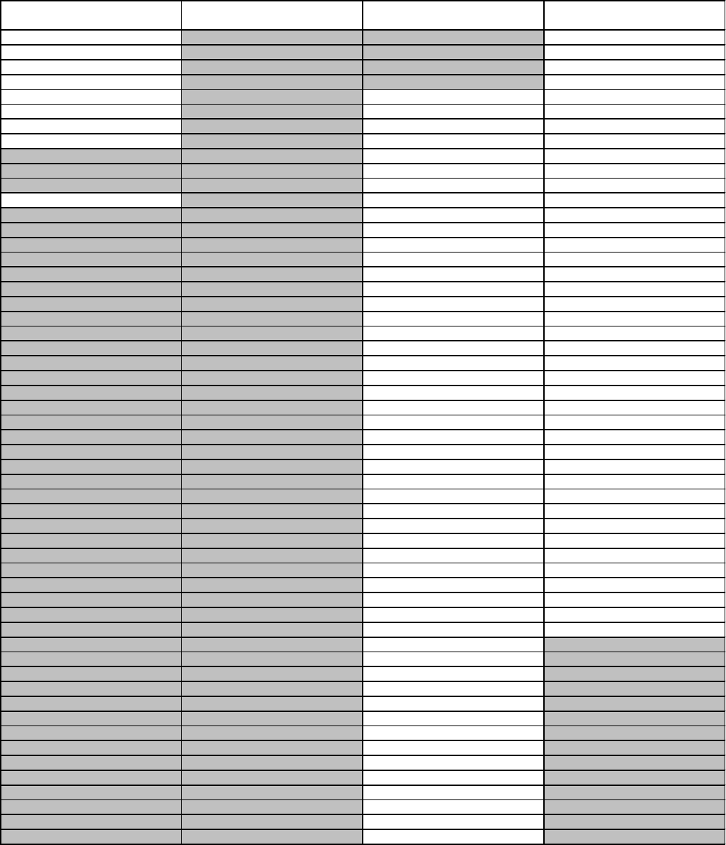
The LTCP-EZ Template: A Planning Tool for CSO Control in Small Communities

State

County

1hr-3mo

(in.)

State

County

1hr-3mo

(in.)

State

County

1hr-3mo

(in.)

State

County

1hr-3mo

(in.)

CT Fairfield 0.87 IL Johnson 0.90 IL Will 0.76 IN Miami 0.71

CT Hartford 0.87 IL Kane 0.76 IL Williamson 0.90 IN Monroe 0.81

CT Litchfield 0.87 IL Kankakee 0.76 IL Winnebago 0.78 IN Montgomery 0.79

CT Middlesex 0.87 IL Kendall 0.76 IL Woodford 0.76 IN Morgan 0.74

CT New Haven 0.87 IL Knox 0.84 IN Adams 0.65 IN Newton 0.73

CT New London 0.87 IL La Salle 0.76 IN Allen 0.65 IN Noble 0.65

CT Tolland 0.87 IL Lake 0.76 IN Bartholomew 0.74 IN Ohio 0.74

CT Windham 0.87 IL Lawrence 0.79 IN Benton 0.73 IN Orange 0.81

DE Kent 0.87 IL Lee 0.78 IN Blackford 0.69 IN Owen 0.79

DE New Castle 0.87 IL Livingston 0.74 IN Boone 0.74 IN Parke 0.79

DE Sussex

0.87 IL Logan 0.76 IN Brown 0.81 IN Perry 0.81

DC DC 0.87 IL Macon 0.76 IN Carroll 0.74 IN Pike 0.83

IL Adams 0.84 IL Macoupin 0.79 IN Cass 0.71 IN Porter 0.73

IL Alexander 0.90 IL Madison 0.81 IN Clark 0.74 IN Posey 0.83

IL Bond 0.81 IL Marion 0.79 IN Clay 0.79 IN Pulaski 0.73

IL Boone 0.78 IL Marshall 0.76 IN Clinton 0.74 IN Putnam 0.79

IL Brown 0.76 IL Mason 0.76 IN Crawford 0.81 IN Randolph 0.69

IL Bureau 0.78 IL Massac 0.90 IN Daviess 0.83 IN Ripley 0.74

IL Calhoun 0.79 IL McDonough 0.84 IN Dearborn 0.74 IN Rush 0.74

IL Carroll 0.78 IL McHenry 0.76 IN Decatur 0.74 IN Scott 0.74

IL Cass 0.79 IL McLean 0.76 IN DeKalb 0.65 IN Shelby 0.74

IL Champaign 0.74 IL

Menard 0.79 IN Delaware 0.69 IN Spencer 0.83

IL Christian 0.79 IL Mercer 0.78 IN Dubois 0.83 IN St. Joseph 0.71

IL Clark 0.77 IL Monroe 0.81 IN Elkhart 0.71 IN Starke 0.73

IL Clay 0.79 IL Montgomery 0.79 IN Fayette 0.69 IN Steuben 0.65

IL Clinton 0.81 IL Morgan 0.79 IN Floyd 0.81 IN Sullivan 0.83

IL Coles 0.77 IL Moultrie 0.77 IN Fountain 0.79 IN Switzerland 0.74

IL Cook 0.76 IL Ogle 0.78 IN Franklin 0.74 IN Tippecanoe 0.79

IL Crawford 0.77 IL Peoria 0.76 IN Fulton 0.71 IN Tipton 0.74

IL Cumberland 0.77 IL Perry 0.81 IN Gibson 0.83 IN Union 0.69

IL De Witt 0.76 IL Piatt 0.76 IN Grant 0.74 IN Vanderburgh 0.83

IL DeKalb 0.76 IL Pike 0.79 IN Greene 0.83 IN Vermillion 0.79

IL Douglas 0.77 IL Pope 0.90

IN Hamilton 0.74 IN Vigo 0.79

IL DuPage 0.76 IL Pulaski 0.90 IN Hancock 0.74 IN Wabash 0.71

IL Edgar 0.77 IL Putnam 0.78 IN Harrison 0.81 IN Warren 0.79

IL Edwards 0.79 IL Randolph 0.81 IN Hendricks 0.74 IN Warrick 0.83

IL Effingham 0.77 IL Richland 0.79 IN Henry 0.69 IN Washington 0.81

IL Fayette 0.77 IL Rock Island 0.78 IN Howard 0.74 IN Wayne 0.69

IL Ford 0.74 IL Saline 0.90 IN Huntington 0.65 IN Wells 0.65

IL Franklin 0.79 IL Sangamon 0.79 IN Jackson 0.81 IN White 0.73

IL Fulton 0.76 IL Schuyler 0.76 IN Jasper 0.73 IN Whitley 0.65

IL Gallatin 0.90 IL Scott 0.79 IN Jay 0.69 IA Adair 0.83

IL Greene 0.79 IL Shelby 0.77 IN Jefferson 0.74 IA Adams 0.83

IL Grundy 0.76 IL St. Clair 0.81 IN Jennings

0.74 IA Allamakee 0.70

IL Hamilton 0.79 IL Stark 0.76 IN Johnson 0.74 IA Appanoose 0.75

IL Hancock 0.84 IL Stephenson 0.78 IN Knox 0.83 IA Audubon 0.75

IL Hardin 0.90 IL Tazewell 0.76 IN Kosciusko 0.71 IA Benton 0.72

IL Henderson 0.84 IL Union 0.90 IN Lagrange 0.65 IA Black Hawk 0.70

IL Henry 0.78 IL Vermilion 0.74 IN Lake 0.73 IA Boone 0.72

IL Iroquois 0.74 IL Wabash 0.79 IN LaPorte 0.73 IA Bremer 0.70

IL Jackson 0.90 IL Warren 0.84 IN Lawrence 0.81 IA Buchanan 0.70

IL Jasper 0.77 IL Washington 0.81 IN Madison 0.74 IA Buena Vista 0.67

IL Jefferson 0.79 IL Wayne 0.79 IN Marion 0.74 IA Butler 0.71

IL Jersey 0.79 IL White 0.79 IN Marshall 0.71 IA Calhoun 0.75

IL Jo Daviess 0.78 IL Whiteside 0.78 IN Martin 0.83 IA

Carroll 0.75

A-1

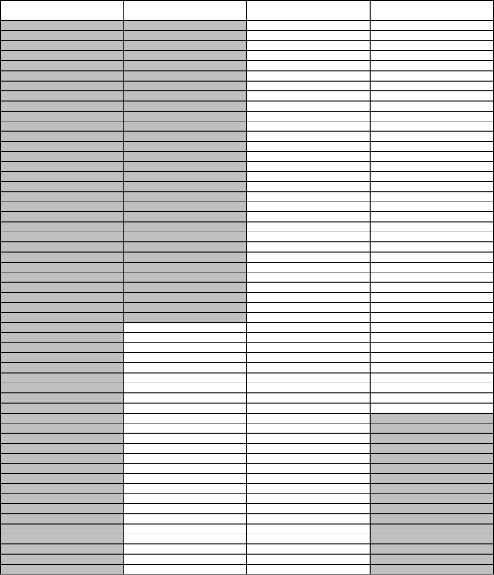
Appendix A: One-Hour Three-Month Rainfall Intensities, SCHEDULE 4 – CSO VOLUME

A-2

State

County

1hr-3mo

(in.)

State

County

1hr-3mo

(in.)

State

County

1hr-3mo

(in.)

State

County

1hr-3mo

(in.)

IA Cass 0.83 IA Muscatine 0.72 KY Clinton 0.88 KY Meade 0.88

IA Cedar 0.72 IA O'Brien 0.67 KY Crittenden 0.93 KY Menifee 0.80

IA Cerro Gordo 0.71 IA Osceola 0.67 KY Cumberland 0.88 KY Mercer 0.77

IA Cherokee 0.67 IA Page 0.83 KY Daviess 0.93 KY Metcalfe 0.88

IA Chickasaw 0.70 IA Palo Alto 0.67 KY Edmonson 0.88 KY Monroe 0.88

IA Clarke 0.75 IA Plymouth 0.67 KY Elliott 0.80 KY Montgomery 0.77

IA Clay 0.67 IA Pocahontas 0.67 KY Estill 0.80 KY Morgan 0.80

IA Clayton 0.70 IA Polk 0.72 KY Fayette 0.77 KY Muhlenberg 0.93

IA Clinton 0.72 IA

Pottawattami

0.83 KY Fleming 0.77 KY Nelson 0.88

IA Crawford 0.75 IA Poweshiek 0.72 KY Floyd 0.80 KY Nicholas 0.77

IA Dallas 0.72 IA Ringgold 0.75 KY Franklin 0.77 KY Ohio 0.93

IA Davis 0.75 IA Sac 0.75 KY Fulton 0.93 KY Oldham 0.77

IA Decatur 0.75 IA Scott 0.72 KY Gallatin 0.77 KY Owen 0.77

IA Delaware 0.70 IA Shelby 0.75 KY Garrard 0.77 KY Owsley 0.80

IA Des Moines 0.75 IA Sioux 0.67 KY Grant 0.77 KY Pendleton 0.77

IA Dickinson 0.67 IA Story 0.72 KY Graves 0.93 KY Perry 0.80

IA Dubuque 0.70 IA Tama 0.72 KY Grayson 0.88 KY Pike 0.80

IA Emmet 0.67 IA Taylor 0.83 KY Green 0.88 KY Powell 0.80

IA Fayette 0.70 IA Union 0.75 KY Greenup 0.80 KY Pulaski 0.80

IA Floyd 0.71 IA Van Buren 0.75 KY Hancock 0.93 KY Robertson 0.77

IA Franklin 0.71 IA Wapello 0.75 KY Hardin 0.88 KY Rockcastle 0.80

IA Fremont 0.83 IA Warren 0.75 KY Harlan 0.80 KY Rowan 0.80

IA Greene 0.75 IA Washington 0.75 KY Harrison 0.77 KY Russell 0.88

IA Grundy 0.72 IA Wayne 0.75 KY Hart 0.88 KY Scott 0.77

IA Guthrie 0.75 IA Webster 0.72 KY Henderson 0.93 KY Shelby 0.77

IA Hamilton 0.72 IA Winnebago 0.71 KY Henry 0.77 KY Simpson 0.93

IA Hancock 0.71 IA Winneshiek 0.70 KY Hickman 0.93 KY Spencer 0.77

IA Hardin 0.72 IA Woodbury 0.75 KY Hopkins 0.93 KY Taylor 0.88

IA Harrison 0.75 IA Worth 0.71 KY Jackson 0.80 KY Todd 0.93

IA Henry 0.75 IA Wright 0.71 KY Jefferson 0.88 KY Trigg 0.93

IA Howard 0.70 KY Adair 0.88 KY Jessamine 0.77

KY Trimble 0.77

IA Humboldt 0.71 KY Allen 0.88 KY Johnson 0.80 KY Union 0.93

IA Ida 0.75 KY Anderson 0.77 KY Kenton 0.77 KY Warren 0.88

IA Iowa 0.72 KY Ballard 0.93 KY Knott 0.80 KY Washington 0.77

IA Jackson 0.72 KY Barren 0.88 KY Knox 0.80 KY Wayne 0.80

IA Jasper 0.72 KY Bath 0.77 KY Larue 0.88 KY Webster 0.93

IA Jefferson 0.75 KY Bell 0.80 KY Laurel 0.80 KY Whitley 0.80

IA Johnson 0.72 KY Boone 0.77 KY Lawrence 0.80 KY Wolfe 0.80

IA Jones 0.72 KY Bourbon 0.77 KY Lee 0.80 KY Woodford 0.77

IA Keokuk 0.75 KY Boyd 0.80 KY Leslie 0.80 ME

Androscoggi

0.75

IA Kossuth 0.71 KY Boyle 0.77 KY Letcher 0.80 ME Aroostook 0.62

IA Lee 0.75 KY Bracken 0.77 KY Lewis 0.80 ME Cumberland 0.75

IA Linn 0.72 KY Breathitt 0.80 KY Lincoln 0.77 ME Franklin 0.75

IA Louisa 0.75 KY Breckinridge 0.88 KY Livingston 0.93 ME Hancock 0.75

IA Lucas 0.75 KY Bullitt 0.88 KY Logan 0.93 ME Kennebec 0.75

IA Lyon 0.67 KY Butler 0.88 KY Lyon 0.93 ME Knox 0.75

IA Madison 0.75 KY Calloway 0.93 KY Madison 0.77 ME Lincoln 0.75

IA Mahaska 0.75 KY Campbell 0.77 KY Magoffin 0.80 ME Oxford 0.87

IA Marion 0.75 KY Carlisle 0.93 KY Marion 0.88 ME Penobscot 0.75

IA Marshall 0.72 KY Carroll 0.77 KY Marshall 0.93 ME Piscataquis 0.75

IA Mills 0.83 KY Carter 0.80 KY Martin 0.80 ME Sagadahoc 0.75

Mitchell 0.71 KY Casey 0.88 KY Mason 0.77 ME Somerset 0.75

IA Monona 0.75 KY Christian 0.93 KY McCracken 0.93 ME Waldo 0.75

IA Monroe 0.75 KY Clark 0.77 KY McCreary 0.80 ME Washington 0.75

IA Montgomery 0.83 KY Clay 0.80 KY McLean 0.93 ME York 0.75

The LTCP-EZ Template: A Planning Tool for CSO Control in Small Communities

A-3

State

County

1hr-3mo

(in.)

State

County

1hr-3mo

(in.)

State

County

1hr-3mo

(in.)

State

County

1hr-3mo

(in.)

MD Allegany 0.75 MI Clare 0.56 MI Saginaw 0.52 MO Howard 0.76

MD Anne Arundel 0.87 MI Clinton 0.61 MI Sanilac 0.52 MO Howell 0.84

MD Baltimore 0.87 MI Crawford 0.51 MI Schoolcraft 0.50 MO Iron 0.84

MD Baltimore City 0.87 MI Delta 0.50 MI Shiawassee 0.61 MO Jackson 0.76

MD Calvert 0.87 MI Dickinson 0.59 MI St. Clair 0.56 MO Jasper 0.90

MD Caroline 0.87 MI Eaton 0.61 MI St. Joseph 0.61 MO Jefferson 0.84

MD Carroll 0.87 MI Emmet 0.49 MI Tuscola 0.52 MO Johnson 0.84

MD Cecil 0.87 MI Genesee 0.56 MI Van Buren 0.59 MO Knox 0.75

MD Charles 0.87 MI Gladwin 0.56 MI Washtenaw 0.56 MO Laclede 0.90

MD Dorchester 0.87 MI Gogebic 0.59 MI Wayne 0.56 MO Lafayette 0.76

MD Frederick

0.87 MI Grand Traverse 0.49 MI Wexford 0.49 MO Lawrence 0.90

MD Garrett 0.75 MI Gratiot 0.56 MO Adair 0.75 MO Lewis 0.75

MD Harford 0.87 MI Hillsdale 0.61 MO Andrew 0.76 MO Lincoln 0.75

MD Howard 0.87 MI Houghton 0.59 MO Atchison 0.76 MO Linn 0.76

MD Kent 0.87 MI Huron 0.52 MO Audrain 0.75 MO Livingston 0.76

MD Montgomery 0.87 MI Ingham 0.61 MO Barry 0.90 MO Macon 0.75

MD Prince George's 0.87 MI Ionia 0.61 MO Barton 0.90 MO Madison 0.84

MD Queen Anne's 0.87 MI Iosco 0.51 MO Bates 0.84 MO Maries 0.84

MD Somerset 1.00 MI Iron 0.59 MO Benton 0.84 MO Marion 0.75

MD St. Mary's 0.87 MI Isabella 0.56 MO Bollinger 0.84 MO McDonald 0.90

MD Talbot 0.87 MI Jackson 0.61 MO Boone 0.75 MO Mercer 0.76

MD Washington 0.75 MI

Kalamazoo 0.59 MO Buchanan 0.76 MO Miller 0.84

MD Wicomico 0.87 MI Kalkaska 0.49 MO Butler 0.84 MO Mississippi 0.90

MD Worcester 1.00 MI Kent 0.59 MO Caldwell 0.76 MO Moniteau 0.84

MA Barnstable 0.87 MI Keweenaw 0.59 MO Callaway 0.75 MO Monroe 0.75

MA Berkshire 0.75 MI Lake 0.53 MO Camden 0.84 MO Montgomery 0.75

MA Bristol 0.87 MI Lapeer 0.56 MO Cape Girardeau 0.84 MO Morgan 0.84

MA Dukes 0.87 MI Leelanau 0.49 MO Carroll 0.76 MO New Madrid 0.90

MA Essex 0.87 MI Lenawee 0.56 MO Carter 0.84 MO Newton 0.90

MA Franklin 0.75 MI Livingston 0.56 MO Cass 0.84 MO Nodaway 0.76

MA Hampden 0.87 MI Luce 0.50 MO Cedar 0.84 MO Oregon 0.84

MA Hampshire 0.75 MI Mackinac 0.50 MO Chariton 0.76 MO Osage 0.75

MA Middlesex 0.87 MI Macomb 0.56

MO Christian 0.90 MO Ozark 0.90

MA Nantucket 0.87 MI Manistee 0.49 MO Clark 0.75 MO Pemiscot 0.90

MA Norfolk 0.87 MI Marquette 0.59 MO Clay 0.76 MO Perry 0.84

MA Plymouth 0.87 MI Mason 0.53 MO Clinton 0.76 MO Pettis 0.84

MA Suffolk 0.87 MI Mecosta 0.56 MO Cole 0.84 MO Phelps 0.84

MA Worcester 0.87 MI Menominee 0.59 MO Cooper 0.84 MO Pike 0.75

MI Alcona 0.51 MI Midland 0.56 MO Crawford 0.84 MO Platte 0.76

MI Alger 0.50 MI Missaukee 0.49 MO Dade 0.90 MO Polk 0.90

MI Allegan 0.59 MI Monroe 0.56 MO Dallas 0.90 MO Pulaski 0.84

MI Alpena 0.51 MI Montcalm 0.56 MO Daviess 0.76 MO Putnam 0.76

MI Antrim 0.49 MI Montmorency 0.51 MO DeKalb 0.76 MO Ralls 0.75

MI Arenac 0.52 MI Muskegon 0.53 MO Dent

0.84 MO Randolph 0.75

MI Baraga 0.59 MI Newaygo 0.53 MO Douglas 0.90 MO Ray 0.76

MI Barry 0.61 MI Oakland 0.56 MO Dunklin 0.90 MO Reynolds 0.84

MI Bay 0.52 MI Oceana 0.53 MO Franklin 0.75 MO Ripley 0.84

MI Benzie 0.49 MI Ogemaw 0.51 MO Gasconade 0.75 MO Saline 0.76

MI Berrien 0.59 MI Ontonagon 0.59 MO Gentry 0.76 MO Schuyler 0.75

MI Branch 0.61 MI Osceola 0.56 MO Greene 0.90 MO Scotland 0.75

MI Calhoun 0.61 MI Oscoda 0.51 MO Grundy 0.76 MO Scott 0.90

MI Cass 0.59 MI Otsego 0.51 MO Harrison 0.76 MO Shannon 0.84

MI Charlevoix 0.49 MI Ottawa 0.59 MO Henry 0.84 MO Shelby 0.75

MI Cheboygan 0.51 MI Presque Isle 0.51 MO Hickory 0.84 MO St. Charles 0.75

MI Chippewa 0.50 MI Roscommon 0.51 MO Holt 0.76 MO

St. Clair 0.84

Appendix A: One-Hour Three-Month Rainfall Intensities, SCHEDULE 4 – CSO VOLUME

A-4

State

County

1hr-3mo

(in.)

State

County

1hr-3mo

(in.)

State

County

1hr-3mo

(in.)

State

County

1hr-3mo

(in.)

MO St. Francois 0.84 NY Chenango 0.75 OH Allen 0.61 OH Montgomery 0.70

MO St. Louis 0.75 NY Clinton 0.62 OH Ashland 0.63 OH Morgan 0.61

MO St. Louis City 0.75 NY Columbia 0.75 OH Ashtabula 0.61 OH Morrow 0.65

MO Ste. Genevieve 0.84 NY Cortland 0.75 OH Athens 0.61 OH Muskingum 0.61

MO Stoddard 0.90 NY Delaware 0.75 OH Auglaize 0.65 OH Noble 0.61

MO Stone 0.90 NY Dutchess 1.00 OH Belmont 0.61 OH Ottawa 0.60

MO Sullivan 0.76 NY Erie 0.62 OH Brown 0.70 OH Paulding 0.61

MO Taney 0.90 NY Essex 0.62 OH Butler 0.70 OH Perry 0.61

MO Texas 0.84 NY Franklin 0.62 OH Carroll 0.61 OH Pickaway 0.65

MO Vernon 0.84 NY Fulton 0.75 OH Champaign 0.65 OH Pike 0.69

Warren 0.75 NY Genesee 0.62 OH Clark 0.65 OH Portage 0.61

MO Washington 0.84 NY Greene 0.87 OH Clermont 0.70 OH Preble 0.70

MO Wayne 0.84 NY Hamilton 0.62 OH Clinton 0.70 OH Putnam 0.61

MO Webster 0.90 NY Herkimer 0.62 OH Columbiana 0.61 OH Richland 0.63

MO Worth 0.76 NY Jefferson 0.62 OH Coshocton 0.63 OH Ross 0.69

MO Wright 0.90 NY Kings 0.87 OH Crawford 0.60 OH Sandusky 0.60

NH Belknap 0.75 NY Lewis 0.62 OH Cuyahoga 0.61 OH Scioto 0.69

NH Carroll 0.87 NY Livingston 0.62 OH Darke 0.65 OH Seneca 0.60

NH Cheshire 0.75 NY Madison 0.75 OH Defiance 0.61 OH Shelby 0.65

NH Coos 0.87 NY Monroe 0.62 OH Delaware 0.65 OH Stark 0.61

NH Grafton 0.75 NY Montgomery 0.75 OH Erie 0.60 OH Summit 0.61

NH Hillsborough 0.75

NY Nassau 0.87 OH Fairfield 0.65 OH Trumbull 0.61

NH Merrimack 0.75 NY New York 0.87 OH Fayette 0.65 OH Tuscarawas 0.61

NH Rockingham 0.75 NY Niagara 0.62 OH Franklin 0.65 OH Union 0.65

NH Strafford 0.75 NY Oneida 0.75 OH Fulton 0.61 OH Van Wert 0.61

NH Sullivan 0.75 NY Onondaga 0.75 OH Gallia 0.69 OH Vinton 0.61

NJ Atlantic 0.87 NY Ontario 0.62 OH Geauga 0.61 OH Warren 0.70

NJ Bergen 0.87 NY Orange 0.87 OH Greene 0.70 OH Washington 0.61

NJ Burlington 0.87 NY Orleans 0.62 OH Guernsey 0.61 OH Wayne 0.63

NJ Camden 0.87 NY Oswego 0.62 OH Hamilton 0.70 OH Williams 0.61

NJ Cape May 0.87 NY Otsego 0.75 OH Hancock 0.61 OH Wood 0.61

NJ Cumberland 0.87 NY Putnam 0.87 OH Hardin 0.65 OH Wyandot 0.60

NJ Essex 0.87 NY Queens

0.87 OH Harrison 0.61 PA Adams 0.75

NJ Gloucester 0.87 NY Rensselaer 0.75 OH Henry 0.61 PA Allegheny 0.75

NJ Hudson 0.87 NY Richmond 0.87 OH Highland 0.70 PA Armstrong 0.75

NJ Hunterdon 0.87 NY Rockland 0.87 OH Hocking 0.61 PA Beaver 0.75

NJ Mercer 0.87 NY Saratoga 0.75 OH Holmes 0.63 PA Bedford 0.75

NJ Middlesex 0.87 NY Schenectady 0.75 OH Huron 0.60 PA Berks 0.87

NJ Monmouth 0.87 NY Schoharie 0.75 OH Jackson 0.69 PA Blair 0.75

NJ Morris 0.87 NY Schuyler 0.75 OH Jefferson 0.61 PA Bradford 0.75

NJ Ocean 0.87 NY Seneca 0.75 OH Knox 0.63 PA Bucks 0.87

NJ Passaic 0.87 NY St. Lawrence 0.62 OH Lake 0.61 PA Butler 0.75

NJ Salem 0.87 NY Steuben 0.75 OH Lawrence 0.69 PA Cambria 0.75

NJ Somerset 0.87 NY Suffolk 0.87 OH

Licking 0.65 PA Cameron 0.75

NJ Sussex 0.87 NY Sullivan 0.87 OH Logan 0.65 PA Carbon 0.75

NJ Union 0.87 NY Tioga 0.75 OH Lorain 0.60 PA Centre 0.75

NJ Warren 0.87 NY Tompkins 0.75 OH Lucas 0.61 PA Chester 0.87

NY Albany 0.75 NY Ulster 1.00 OH Madison 0.65 PA Clarion 0.75

NY Allegany 0.75 NY Warren 0.62 OH Mahoning 0.61 PA Clearfield 0.75

NY Bronx 0.87 NY Washington 0.75 OH Marion 0.65 PA Clinton 0.75

NY Broome 0.75 NY Wayne 0.62 OH Medina 0.61 PA Columbia 0.75

NY Cattaraugus 0.75 NY Westchester 0.87 OH Meigs 0.69 PA Crawford 0.62

NY Cayuga 0.75 NY Wyoming 0.62 OH Mercer 0.65 PA Cumberland 0.75

NY Chautauqua 0.62 NY Yates 0.75 OH Miami 0.65 PA Dauphin 0.75

NY Chemung 0.75 OH Adams 0.69 OH Monroe 0.61

PA Delaware 0.87

The LTCP-EZ Template: A Planning Tool for CSO Control in Small Communities

State

County

1hr-3mo

(in.)

State

County

1hr-3mo

(in.)

State

County

1hr-3mo

(in.)

State

County

1hr-3mo

(in.)

Elk 0.75 VT Grand Isle 0.62 VA Hanover 0.87 VA Suffolk 1.00

PA Erie 0.62 VT Lamoille 0.62 VA Henrico 0.87 VA Surry 1.00

PA Fayette 0.75 VT Orange 0.62 VA Henry 1.00 VA Sussex 1.00

PA Forest 0.75 VT Orleans 0.62 VA Highland 0.75 VA Tazewell 0.75

Franklin 0.75 VT Rutland 0.75 VA Hopewell 0.87 VA Virginia Beach 1.00

PA Fulton 0.75 VT Washington 0.62 VA Isle of Wight 1.00 VA Warren 1.00

PA Greene 0.75 VT Windham 0.75 VA James City 1.00 VA Washington 0.75

PA Huntingdon 0.75 VT Windsor 0.75 VA King and Queen 0.87 VA Westmoreland 0.87

Indiana 0.75 VA Accomack 1.00 VA King George 0.87 VA Williamsburg 1.00

PA Jefferson 0.75 VA Albemarle 1.00 VA King William 0.87 VA Wise 0.75

PA Juniata 0.75 VA Alexandria 0.87 VA Lancaster 0.87 VA Wythe 0.75

PA Lackawanna 0.75 VA Alleghany 0.75 VA Lee 0.75 VA York 1.00

Lancaster 0.87 VA Amelia 0.87 VA Loudoun 0.87 WV Barbour 0.75

PA Lawrence 0.62 VA Amherst 1.00 VA Louisa 0.87 WV Berkeley 0.75

PA Lebanon 0.75 VA Appomattox 1.00 VA Lunenburg 0.87 WV Boone 0.75

PA Lehigh 0.87 VA Augusta 1.00 VA Lynchburg 1.00 WV Braxton 0.75

Luzerne 0.75 VA Bath 0.75 VA Madison 1.00 WV Brooke 0.75

PA Lycoming 0.75 VA Bedford 1.00 VA Manassas 0.87 WV Cabell 0.75

PA McKean 0.75 VA Bland 0.75 VA Manassas Park 0.87 WV Calhoun 0.75

PA Mercer 0.62 VA Botetourt 1.00 VA Mathews 1.00 WV Clay 0.75

Mifflin 0.75 VA Brunswick 0.87 VA Mecklenburg 0.87 WV Doddridge 0.75

PA Monroe 0.75

VA Buchanan 0.75 VA Middlesex 0.87 WV Fayette 0.75

PA Montgomery 0.87 VA Buckingham 1.00 VA Montgomery 0.87 WV Gilmer 0.75

PA Montour 0.75 VA Campbell 1.00 VA Nelson 1.00 WV Grant 0.75

Northampton 0.87 VA Caroline 0.87 VA New Kent 0.87 WV Greenbrier 0.75

PA Northumberland 0.75 VA Carroll 0.87 VA Newport News 1.00 WV Hampshire 0.75

PA Perry 0.75 VA Charles City 0.87 VA Norfolk 1.00 WV Hancock 0.75

PA Philadelphia 0.87 VA Charlotte 0.87 VA Northampton 1.00 WV Hardy 0.75

Pike 0.75 VA Chesapeake 1.00 VA Northumberland 0.87 WV Harrison 0.75

PA Potter 0.75 VA Chesterfield 0.87 VA Nottoway 0.87 WV Jackson 0.75

PA Schuylkill 0.75 VA Clarke 0.87 VA Orange 1.00 WV Jefferson 0.87

PA Snyder 0.75 VA Colonial Heights 0.87 VA Page 1.00 WV Kanawha 0.75

Somerset 0.75 VA Craig 0.75 VA Patrick 1.00 WV Lewis 0.75

PA Sullivan 0.75 VA Culpeper 1.00 VA Petersburg 0.87 WV Lincoln 0.75

PA Susquehanna 0.75 VA Cumberland 0.87 VA Pittsylvania 0.87 WV Logan 0.75

PA Tioga 0.75 VA Dickenson 0.75 VA Poquoson 1.00 WV Marion 0.75

Union 0.75 VA Dinwiddie 0.87 VA Portsmouth 1.00 WV Marshall 0.75

PA Venango 0.75 VA Essex 0.87 VA Powhatan 0.87 WV Mason 0.75

PA Warren 0.75 VA Fairfax 0.87 VA Prince Edward 0.87 WV McDowell 0.75

PA Washington 0.75 VA Fairfax City 0.87 VA Prince George 0.87 WV Mercer 0.75

Wayne 0.75 VA Falls Church 0.87 VA Prince William 0.87 WV Mineral 0.75

PA Westmoreland 0.75 VA Fauquier 1.00 VA Pulaski 0.75 WV Mingo 0.75

PA Wyoming 0.75 VA Floyd 0.87 VA Rappahannock 1.00 WV Monongalia 0.75

PA York 0.87 VA Fluvanna 1.00 VA Richmond 0.87 WV Monroe 0.75

Bristol 0.87 VA Franklin 1.00 VA Richmond City 0.87 WV Morgan 0.75

RI Kent 0.87 VA Frederick 0.75 VA Roanoke 1.00 WV Nicholas 0.75

RI Newport 0.87 VA Fredericksburg 0.87 VA Rockbridge 1.00 WV Ohio 0.75

Providence 0.87 VA Giles 0.75 VA Rockingham 1.00 WV Pendleton 0.75

Washington 0.87 VA Gloucester 1.00 VA Russell 0.75 WV Pleasants 0.75

VT Addison 0.62 VA Goochland 0.87 VA Scott 0.75 WV Pocahontas 0.75

VT Bennington 0.75 VA Grayson 0.75 VA Shenandoah 0.87 WV Preston 0.75

VT Caledonia 0.62 VA Greene 1.00 VA Smyth 0.75 WV Putnam 0.75

VT Chittenden 0.62 VA Greensville 1.00 VA Southampton 1.00 WV Raleigh 0.75

VT Essex 0.62 VA Halifax 0.87 VA Spotsylvania 0.87 WV Randolph 0.75

VT Franklin 0.62 VA Hampton 1.00 VA Stafford 0.87

WV Ritchie 0.75

A-5

Appendix A: One-Hour Three-Month Rainfall Intensities, SCHEDULE 4 – CSO VOLUME

A-6

State

County

1hr-3mo

(in.)

State

County

1hr-3mo

(in.)

WV Roane 0.75 WI Oneida 0.67

WV Summers 0.75

WI Outagamie 0.59

WV Taylor 0.75 WI Ozaukee 0.65

WV Tucker 0.75 WI Pepin 0.67

WV Tyler

0.75 WI Pierce 0.67

WV Upshur 0.75 WI Polk 0.67

WV Wayne 0.75

WI Portage 0.65

WV Webster 0.75 WI Price 0.67

WV Wetzel 0.75 WI Racine 0.65

WV Wirt

0.75 WI Richland 0.68

WV Wood 0.75 WI Rock 0.68

WV Wyoming 0.75

WI Rusk 0.67

WI Adams 0.65 WI Sauk 0.68

WI Ashland 0.67 WI Sawyer 0.67

WI Barron

0.67 WI Shawano 0.57

WI Bayfield 0.67 WI Sheboygan 0.59

WI Brown 0.59

WI St. Croix 0.67

WI Buffalo 0.67 WI Taylor 0.67

WI Burnett 0.67 WI Trempealeau 0.67

WI Calumet

0.59 WI Vernon 0.68

WI Chippewa 0.67 WI Vilas 0.67

WI Clark

0.67

WI Walworth 0.65

WI Columbia 0.68 WI Washburn 0.67

WI Crawford 0.68 WI Washington 0.65

WI Dane

0.68 WI Waukesha 0.65

WI Dodge 0.68 WI Waupaca 0.65

WI Door 0.59

WI Waushara 0.65

WI Douglas 0.67 WI Winnebago 0.59

WI Dunn 0.67 WI Wood 0.65

WI Eau Claire

0.67

WI Florence 0.57

WI Fond Du Lac 0.59

WI Forest 0.57

WI Grant 0.68

WI Green 0.68

WI Green Lake 0.65

WI Iowa 0.68

WI Iron 0.67

WI Jackson 0.67

WI Jefferson 0.68

WI Juneau 0.65

WI Kenosha 0.65

WI Kewaunee 0.59

WI La Crosse 0.67

WI Lafayette 0.68

WI Langlade 0.57

WI Lincoln 0.67

WI Manitowoc 0.59

WI Marathon 0.67

WI Marinette 0.57

WI Marquette 0.65

WI Menominee 0.57

WI Milwaukee 0.65

WI Monroe 0.67

WI Oconto 0.57

Appendix B

HYDRAULIC CALCULATIONS WITHIN LTCP-EZ SCHEDULE 4 – CSO VOLUME AND

SCHEDULE 5 CSO CONTROL

The LTCP-EZ Template: A Planning Tool for CSO Control in Small Communities

Introduction

It is necessary to make several important estimates within Schedule 4: CSO Volume. These estimates are for

quantification of the amount of combined sewage that overflows, the amount of combined sewage that is

diverted to an interceptor and transported to the WWTP, and, in some instances, the amount of combined

sewage that goes untreated at the WWTP. Continuous simulation hydrology and hydraulic models like SWMM

are often applied for these purposes. However, in the spirit of keeping LTCP-EZ easy, simple relationships and

equations were utilized instead of detailed models. This Appendix describes the method used to make these

estimations within the LTCP-EZ Template.

Overflow Fraction of Combined Sewage

The fraction of runoff volume that overflows at the CSO hydraulic control at the lower end of a sub-sewershed

is dependent on peak flow rate within the sub-sewershed (runoff plus dry weather flow) and the hydraulic

control capacity. The peak runoff rate (Q

) for the one-hour, three-month rainfall is calculated with the rational

method. Similarly, the total volume of runoff (V

) for the 24-hour, three-month rainfall is also calculated with the

rational method. The peak runoff rate is compared with the capacity of the hydraulic control to determine

whether or not an overflow occurs. The volume of overflow (V

) depends on the shape of the runoff hydrograph

through the 24-hour rainfall period.

Dimensional reasoning suggests that the ratio of overflow volume to total runoff volume is a function of the

ratio of hydraulic control capacity to the peak runoff rate. It can be shown that, for a triangular hydrograph, the

following relationship holds:

⎟

⎠

⎞

⎜

⎝

⎛

−=

(1)

where V

= volume of overflow (MG);

= total volume of runoff (MG);

= hydraulic control or pump station capacity (MGD); and

= peak runoff rate (MGD).

The overflow fraction of combined sewage in Schedule 4: CSO Volume is defined as the ratio of overflow

volume to total volume, and is calculated as follows:

⎟

⎠

⎞

⎜

⎝

⎛

−=

(2)

where f

= overflow fraction of combined sewage [--].

The actual overflow volume is then computed as follows:

= f

(3)

The situation from which Equation 1 was derived is depicted in Figure 1. Empirical studies show that actual

runoff hydrographs are likely to be shaped more “concave up” relative to the triangular assumption, so that the

fraction of overflow volu

me would be less than that predicted with Equation 1. To test this, the RUNOFF block

within the SWMM Model was used to generate runoff hydrographs from design storms of various lengths, and

for a variety of catchment characteristics. A series of fractional overflow volumes were then computed from the

resulting hydrographs by varying the hydraulic control flow rate, and the fractional volumes were compared

B-1

Appendix B: Hydraulic Calculations within LTCP-EZ SCHEDULE 4 – CSO VOLUME and SCHEDULE 5 – CSO CONTROL

with Equation 1. Three sets of catchments (designated as set A, set B, and set C) were used. These

catchments represent a wide range of CSO subsewershed conditions and are representative of the co

nditions

that would typically be found in a CSO community. Set A consisted of 161 catchments with areas ranging from

2.7 to 174 acres, and ground slopes ranging from 0.0002 to 0.0173. Set B consisted of 161 catchments with

areas ranging from 0.3 to 37 acres, and ground slopes ranging from 0.0024 to 0.129. Set C consisted of 101

catchments with areas ranging from 16 to 4630 acres, and ground slopes ranging from 0.004 to 0.100. The

results are depicted in Figure 2, which shows that the observed ratios of overflow volume (represented by th

individual points) are below the predicted ratios of overflow volume for all regulator flow/peak flow ratios

(represented by the solid line). This suggests that the use of Equation 1 will provide conservative estima

tes of

the volume of overflow at a CSO hydraulic control.

It should be noted that the model results from this te

st are dependent on the assumed shape of the design

storm hyetograph. This test and the SWMM Model application were based on the third quartile distribution o

heavy rainfall at a point, taken from Table 10 of “Rainfall Frequency Atlas of the Midwest” (Huff and Angel,

1992). Use of rainfall at a point was considered appropriate for the relatively small sewersheds of LTCP-EZ

permittees (less than 1,000 acres). The third quartile distribution is specified for storms of 12 to 24 hours.

Diversion Fraction of Combined Sewage

It is intuitive that the volume of runoff diverted to

the interceptor and the WWTP is the difference between the

total volume of runoff and the volume that overflows. However, if the estimate of overflow volume is

conservatively high (using Equation 1), then calculating diversion by subtraction (that is, 1-Equation 1

) will tend

to underestimate the volume diverted. An alternate approach called the Hyetograph Approach was developed

to determine a better and more conservative estimate of the fraction of runoff diverted to the interceptor and

the WWTP. The Hyetograph Approach is also based on the ratio of hydraulic control capacity to peak runoff

rate. It is recognized that a small degree of “double counting” occurs when the two approaches are used

together. That is, the total estimated overflow plus the total estimated conveyance slightly exceeds the tot

runoff plus dry weather sanitary flow. This is acceptable, however, in that it provides a conservative estimate

for both quantities, rather than forcing one quantity to be conservative at the expense of the other.

The Hyetograph Approach assumes that the runoff hydrograph has the same shape as the rainfall h

yetograph,

and that the total volume diverted is simply the sum of the volumes less than Q

added up over the course of

the storm. This concept is graphically depicted in Figure 3, and it was tested with a simple spreadsheet mode

The hyetograph is again the third quartile distribution of heavy rainfall at a point. Fractional volumes were

quantified with a simple spreadsheet model for a range of Q

ratios, and these results are shown in Figu

re 4

as the Hyetograph Approach. Rather than developing a regression equation from the results, a lookup table

was compiled for inclusion in the LTCP-EZ form, and reproduced here as Table 1. For comparison, Figure 4

also shows the diverted fraction of runoff that would be calculated based on 1- Equation 1.

Fraction of Combined Sewage Untreated at WWTP

Similar to what occurs at a CSO hydraulic control, the fractio

n of combined sewage that overflows at the

WWTP is dependent on the peak rate of sewage delivered to the WWTP and the primary treatment capac

ity at

the WWTP. The estimate of combined sewage that overflows or is untreated at the WWTP (V

) is also based

on Equation 1, but with V

equal to the total volume of sewage conveyed to the WWTP during the 24-hour

rainfall event, Q

equal to primary treatment capacity at the WWTP, and Q

equal to the peak rate of sewag

delivered to the WWTP. Use of Equation 1 for this estimation is also thought to be conservative in that it migh

slightly overestimate rather than underestimate the volume of combined sewage untreated at the WWTP.

B-2

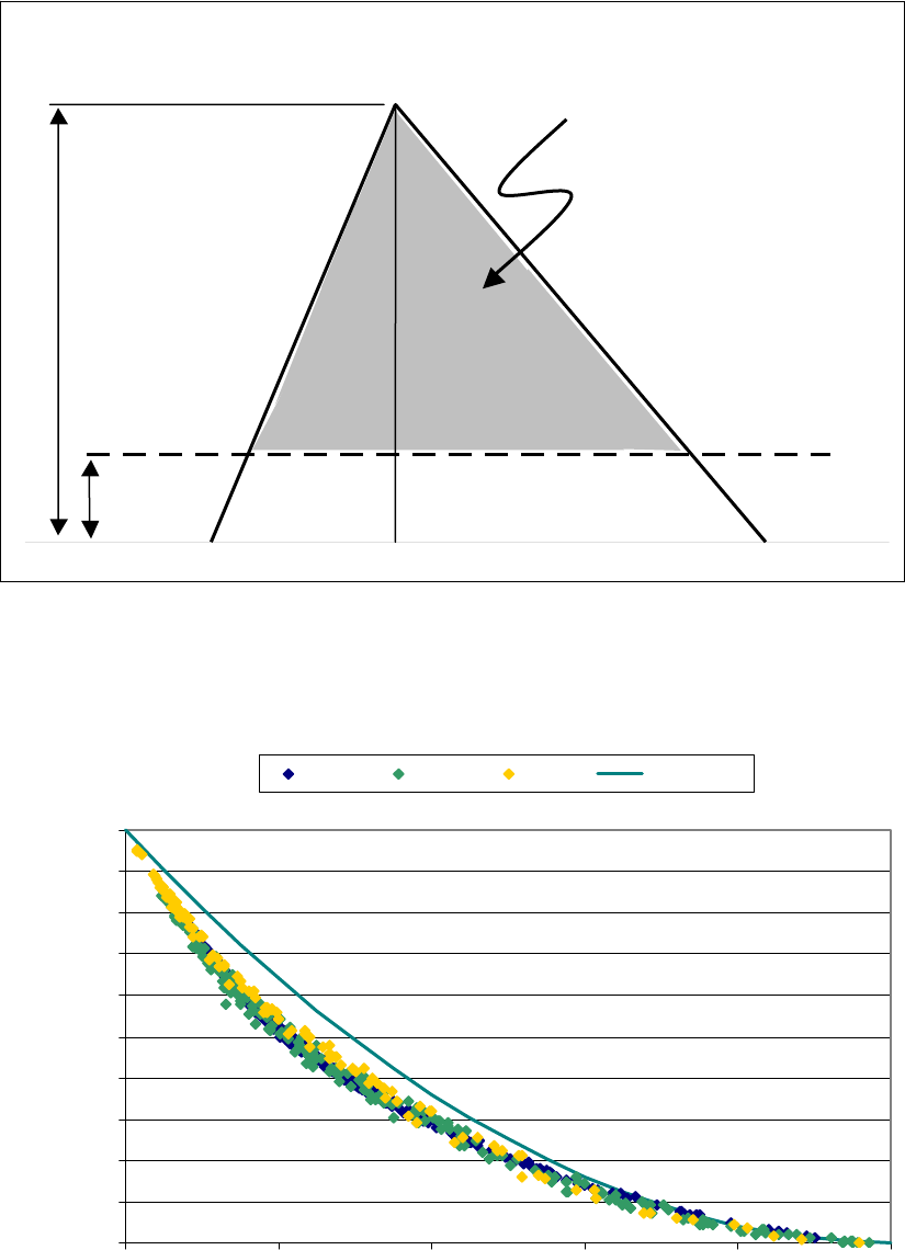
The LTCP-EZ Template: A Planning Tool for CSO Control in Small Communities

Figure 1. Conceptual Diagram of Triangular Runoff Hydrograph

regulator

overflow

peak

Figure 2. Comparison of SWMM Simulated Overflow Volumes with Equation 1.

0.1

0.2

0.3

0.4

0.5

0.6

0.7

0.8

0.9

0 0.2 0.4 0.6 0.8 1

Qregulator/Qpeak

Voverflow/Vtotal

set A set B set C equation 1

B-3

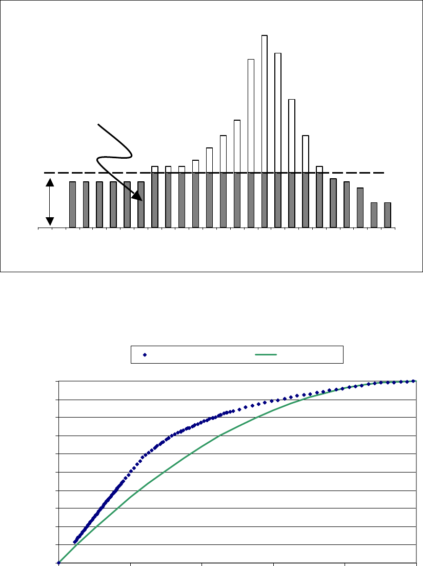
Appendix B: Hydraulic Calculations within LTCP-EZ SCHEDULE 4 – CSO VOLUME and SCHEDULE 5 – CSO CONTROL

Figure 3. Conceptual Diagram of Calculation of Fraction Diverted

1 3 5 7 9 11131517192123

storm hour

Qregulator

Volum e conveyed is sum of

gray colum ns

Figure 4. Comparison of Fraction Conveyed by Hyetograph Approach versus Equation 1

0.1

0.2

0.3

0.4

0.5

0.6

0.7

0.8

0.9

0 0.2 0.4 0.6 0.8 1

Qregulator/Qpeak

Vconveyed/Vtotal

hyetograph approach 1 - equation 1

B-4

The LTCP-EZ Template: A Planning Tool for CSO Control in Small Communities

B-5

Table 1. Fraction of Total Flow Diverted to WWTP from 24-Hour Rainfall

Ratio of Hydraulic control

Capacity to Peak Flow

Rate

Diversion Fraction

0.01 to 0.02 0.04

0.02 to 0.03 0.06

0.03 to 0.04 0.09

0.04 to 0.05 0.11

0.05 to 0.06 0.14

0.06 to 0.07 0.16

0.07 to 0.08 0.19

0.08 to 0.09 0.21

0.09 to 0.10 0.24

0.10 to 0.12 0.28

0.12 to 0.14 0.33

0.14 to 0.16 0.38

0.16 to 0.18 0.42

0.18 to 0.20 0.47

0.20 to 0.24 0.54

0.24 to 0.28 0.62

0.28 to 0.32 0.68

0.32 to 0.36 0.72

0.36 to 0.40 0.76

0.41 to 0.50 0.81

0.51 to 0.60 0.87

0.61 to 0.70 0.91

0.71 to 0.80 0.95

0.81 to 0.90 0.98

0.91 to 1.00 0.99

Appendix C

COST ESTIMATE FOR LTCP-EZ TEMPLATE,

SCHEDULE 5 – CSO CONTROL

The LTCP-EZ Template: A Planning Tool for CSO Control in Small Communities

This Appendix summarizes some of the cost estimate figures used in the LTCP-EZ Template

Schedule 5 – CSO CONTROLS. Localized and/or site-specific costs should be used when they

are available, as localized data will give the most reliable results. However, EPA recognizes that

localized cost data will not always be available, and therefore EPA has provided several cost

estimates based on national data. Descriptions of how these cost estimates were derived are

provided below.

Line 5 –Unit cost of primary treatment per MGD

EPA’s document “Cost of Urban Storm Water Control” (EPA 600/R-02/021), January 2002, uses

the following equation to estimate construction costs for off-line storage areas:

C = 2980V

0.62

Where

C = construction cost ($ millions), in 1999 dollars

V = volume of storage system, in MG

The document indicates that this calculation is valid where 0.15 MG < volume < 30 MG

In addition to this equation, one cost value was collected from the literature. This cost is

summarized below:

1. Chamber Creek WWTP $433,500/MG for primary treatment.

http://www.co.pierce.wa.us/xml/services/home/environ/planning/Appendix%20I.pdf

Line 12 - Average roof area of residential dwellings

The Greenbuilder.com website gave charts showing roof sizes from 1,000 – 2,500 ft

, which is a

good range for residential roof area.

Line 15 – Unit cost per dwelling for residential inflow reduction

Residential inflow reduction is handled in many different ways by different municipalities, leading

to disparities in costs quoted for various reduction measures. Some communities rely on the

homeowner to disconnect downspouts and redirect sump pumps (i.e., Milwaukee, Dearborn,

Indianapolis), and these cost estimates tend to be lower than cost estimates for municipalities

that do the work themselves (Detroit, Toronto). Costs for several downspout disconnection

programs are summarized below:

Downspout disconnection

1. Dearborn, MI – up to $60/household reimbursement for residents doing it themselves.

http://www.rougeriver.com/restoration/projDetail.cfm?ProjectID=780&CategoryID=10

2. Bremerton, WA - $25-$500/household reimbursement for voluntary disconnection,

depending on complexity.

http://www.ci.kenmore.wa.us/html/projects/SedimentaryStudy/Section6Management

Strategies.pdf

3. Portland, OR - $63/downspout.

C-1

Appendix C: Cost Estimate for LTCP-EZ Template, SCHEDULE 5 – CSO CONTROL

4. Indianapolis encourages residents to do it themselves and indicates it should cost less

than $100 apiece.

http://www.indygov.org/eGov/City/DPW/Environment/CleanStream/Help/Residents/

Connect/qa.htm

5. Milwaukee MSD - $15/downspout.

http://www.mmsd.com/programs/downspout_disconnection.cfm

6. Kenmore, WA - $150-$300 per downspout if the city performs the work; $15 if the

homeowner does it.

http://www.ci.kenmore.wa.us/html/projects/SedimentaryStudy/Section6Management

Strategies.pdf

7. Lynn, MA - $20/downspout reimbursement.

http://www.cdm-mich.com/AA-SSO/Public/FinalReport_6_01/Appendix%20M.pdf

8. Elkhart, IN - $150.

http://www.elkhartindiana.org/department/division.asp?fDD=39-203

9. South Bend, Indiana - $150/property

http://www.southbendin.gov/doc/Press_051805_downs.pdf

10. Vancouver, BC – City provided $100/downspout disconnected.

http://www.cityfarmer.org/downspout96.html

11. Detroit, Michigan - $243-$278/property.

http://www.wadetrim.com/resources/pub_conf_downspout.pdf (URL no longer available)

Secondary source: http://www.mmsd.com/stormwaterweb/PDFs/Appendix_L.pdf

12. Toronto, Ontario - $180-$220/property.

http://www.ene.gov.on.ca/envision/gp/4224e_2.htm

Summary: Downspout disconnection costs an approximate average of $100/property if

municipalities have residents do it themselves and $250/property if municipalities do it.

Sump pump redirection

1. Lexington, KY - $1,700/residence.

http://www.lfucg.com/newsreleases/newsreleases/nr_041404.asp

2. Lynn, MA - $500/residence.

http://www.cdm-mich.com/AA-SSO/Public/FinalReport_6_01/Appendix%20M.pdf

Footing Drain Redirection

1. Garden City, MI - $2,000. Other SE Michigan projects have been between $500 and

$6,000/home.

http://www.wadetrim.com/resources/articles/footing_drn.htm (URL no longer available)

2. Duluth, MN – rebate of $1,800/home.

http://www.metrocouncil.org/Environment/ProjectTeams/I-I-tool-box.pdf

3. Twin Cities, MN - $500 - $2,000.

http://www.metrocouncil.org/Environment/ProjectTeams/I-I-tool-box.pdf

4. West Lafayette, IN - $3,500 per building.

http://www.cdm-mich.com/AA-SSO/Public/FinalReport_6_01/Appendix%20M.pdf

C-2

The LTCP-EZ Template: A Planning Tool for CSO Control in Small Communities

5. Auburn Hills, MI - $5,000 per building.

http://www.cdm-mich.com/AA-SSO/Public/FinalReport_6_01/Appendix%20M.pdf

6. Riverview, MI - $5,700 per building.

http://www.cdm-mich.com/AA-SSO/Public/FinalReport_6_01/Appendix%20M.pdf

7. Cedar Rapids, IA - $3,500 per building.

http://www.cdm-mich.com/AA-SSO/Public/FinalReport_6_01/Appendix%20M.pdf

8. Ann Arbor - $3,700 per building.

http://www.cdm-mich.com/aa-fdd/packet.htm

Line 21 – Unit cost for separation per acre

Costs/acre of sewer separated:

1. Seaford, DE: $1,750

2. Skokie/Wilmette, IL: $31,397

3. St. Paul, MN: $17,730

4. Portland, OR: $19,000

5. Providence, RI: $81,000

These costs came from EPA’s Report to Congress: Impacts and Control of CSOs and SSOs,

August 2004 (EPA 833-R-04-001).

6. Portland Maine - $7,352

($5M for 680 acres)

http://www.al

cosan.com/public/WCCP/appendices.pdf

7. Nashville Phase I – $37,910 ($6,634,372 for 175 acres)

http://www.atlantaga.gov/client_resources/mayorsoffice/special%20reports-archive/

csositev.pdf

8. Nashville Phase II – $23,909 ($12,552,277 for 525 acres)

http://www.atlantaga.gov/client_resources/mayorsoffice/special%20reports-archive/

csositev.pdf

9. Boston – ranged from $60,000/acre for partially separated residential neighborhoods to

$190,000/acre for completely combined downtown.

http://books.nap.edu/books/0309048265/html/357.html

10. Atlanta - $41,000/acre.

http://georgia.sierraclub.org/atlanta/conservation/mcwapfin.pdf

11. DCWASA - $360,000/acre.

http://www.dcwasa.com/news/publications/Ops%20Minutes%20July%202004.pdf

Summary: Sewer separation costs an average of approximately $40,000/acre. This cost can

be higher if the area to be separated is in a congested downtown.

Sewer separation costs per linear foot of sewer separated:

1. Harbor Brook and Clinton sewer separation projects, Syracuse, NY, 2000. Cost was

$2,311,126 for 3812 feet of separated pipe, or $606/ft.

http://www.lake.onondaga.ny.us/olpdf/ol303ad.pdf

C-3

Appendix C: Cost Estimate for LTCP-EZ Template, SCHEDULE 5 – CSO CONTROL

C-4

2. Rouge River project - $175-$220/ft (CSO and SSO)

3. Portsmouth, NH - ~$500/ft (personal communication with Peter Rice, City of

Portsmouth).

Line 24 Unit cost per MG of stor

age

EPA’s document “Cost of Urban Storm Water Control” (EPA 600/R-02/021), January, 2002,

uses the following equation to estimate construction costs for off-line storage areas:

C = 4.546V

0.826

Where

C = construction cost ($ millions), in 1999 dollars

V = volume of storage system, in MG

The document indicates that this calculation is valid where 0.15 MG < volume < 30 MG.

In addition to this equation, a number of cost values were collected from the literature. These

are summarized below:

1. EPA’s Report to Congress: Impacts and Control of CSOs and SSOs, August 2004 (EPA

833-R-04-001). Costs per MG of near surface storage ranged from <$0.10 to

$4.61/gallon, with an average of $1.75 gallon.

2. EPA Combined Sewer Overflow Technology Fact Sheet: Retention Basins (EPA 832-F-

99-032). Costs range from $0.32 to $0.98/gallon.

3. Decatur McKinley - $1.09/gallon.

http://books.nap.edu/openbook/0309048265/gifmid/363.gif

4. Decatur 7

Ward – $0.76/gallon.

http://books.nap.edu/openbook/0309048265/gifmid/363.gif

5. Rouge River – range from $2.86 to $8.53/gallon of storage for aboveground facilities.

The average was $5.18/gallon.

http://www.rougeriver.com/cso/overview.html

6. Driftwood Detention Basin, Nashville - $1.96/gallon.

http://www.nashvilleoap.com/projects/driftwood.html

7. San Francisco - $2.35/gallon.

http://www.swrcb.ca.gov/rwqcb2/Agenda/07-16-03/07-16-03-fsheetattachments.doc

Summary: On average, near surface storage costs $2.00 per gallon of storage.